Development of Rainfall Intensity Duration Frequency (IDF) Curves for Hydraulic Design Aspect
Rainfall is one of the major parts that constitute the hydrological cycle, when the rain falls on a built-up area, the water flowing over that area is known as storm water. The storm is characterized mainly by: Intensity, Duration and Frequency. Due to production of greenhouse gases, hydrologic cycle is changing day by day which is causing variations in terms of intensity, duration and frequency of rainfall events. By pinpointing the potential effects of climate change and adapting to them, is the one way to reduce regions susceptibility. Since rainfall characteristics are often used for planning and design of various water resources project, reviewing and bring up-to-date rainfall characteristics which is Intensity–Duration– Frequency (IDF) curves for future climate situations is important. The main objective of this study is to establish the empirical equations of rainfall intensity which can be used in the Upper Nyabarongo catchment (NNYU) for hydraulic structures design. It was found that intensity of rainfalls decreases with increase in rainfall duration. Further, a rainfall of any given duration will have a larger intensity if its return period is large. In other words, for a rainfall for a given duration, rainfalls of higher intensity in that duration are infrequent than rainfalls of smaller intensity.
Twagirayezu Gratien1, Marie Judith Kundwa*2, Philippe
Bakunzibake1, Parfait Bunani3 and Jean Luc Habyarimana3
China
Lanzhou Jiaotong University, China
kudith04@yahoo.fr
the case in Rwandan country. There is high amount of rainfall currently and these increases have a considerable impact on the hydraulic design. For instance, road drainage design was not based on maximum probable flood strategy nor taking high return period. The issue that was identified is that high capacity of runoff overtopped the banks of the channels. Other consequences being more soil erosion caused by one rainstorm of high intensity than by several storms of low intensity. Rainfall intensity (i) is an expression of the rate of rainfall (the most units used are millimeters per hour (mm/hr.)) [1]. In order to plot the amount of water falling within a given period of time, The Intensity - Duration- Frequency (IDF) are used [2, 3, 4]. Rwanda is a country located in the tropical region of the planet. Engineers predicted that it is difficult to construct the IDF curves for precipitation in the above climatic region due to the lack of long –term extreme precipitation data. Careful arrangement is adopted making a combination of limited high frequency information on rain fall peak values with long-term daily information of rainfall. Even tough, it is the case rainfall parameters including its intensity should be determined. And remember that due to climate change, precipitation increased at an alarming rate, and that sudden increase is the primary cause of floods. Flood is one of the most disasters that affect public health and economy worldwide. For the case of Rwanda, because of its geographical features (relief) and climatic profile, it is one of the sub-Saharan countries susceptible to disasters more frequently localized floods [5]. Rwanda is facing the problem of landslides, floods due to rainfall extremes. For such an issue, so many lives of vulnerable citizens were lost, destruction of public & private property, erosion and other kinds of environmental degradation had been prevalent. The major problem was how the rainfall had been managed; because it’s conversion into high discharging runoffs had provoked hydrological problems to deal with [5]. To handle these problems in Rwanda by establishing intensity, duration and frequency curves and their respective empirical equations in order to deal with rainfall changes for different return periods (years). These curves can also be used to determine when an area will be flooded and when a certain rainfall rate or a specific volume of flow will be occurred again in the future. Engineers must be able to quantify rainfall in order to design the proper structures with the collection, conveyance, and storage of excess rainfall. The hydrological aspects of Rwanda, a country of thousand hills is very interesting, therefore the study of the Intensity -duration-frequency –curves will enable to design hydraulic structures for long period of time especially for a study area of upper Nyabarongo catchment. The information is required for water resources projects, sewer systems design, or water quality management projects in large urban areas such as Kigali [6]. Quantification of rainfall is generally done using intensity-duration-frequency (IDF) Curves [7]. This project will be involved in the development of intensity- duration and frequency curves in order to solve problems related to hydraulic design.
Materials and Methods
To achieve the objectives of this research by determining the intensity-duration-frequency curves for Rwanda in the upper Nyabarongo Catchment in order to generate empirical equations of rainfall intensity within the study area. Different materials and methods were used.
Intensity Duration Frequency curves
The rainfall intensity-duration-frequency relationship is one of the most widely used methods in urban drainage design and flood plain management. The establishment of such relationships goes back to as early as 1928 [8]. After Meyer had developed a few, Sherman [9] derived applicable general intensity duration formula to other localities, and Bernard [10] made available for localities within the limits of the study, rainfall intensity formulas for frequencies of 5, 10, 15, 25, 50 and 100 year, applicable to rainfall duration of 120 to 6000 min. In 1935 David Yarn ell made the first intensity –frequency maps for United State. The most known and valuable contribution to the rainfall frequency analysis occurred in TP-40(Technical Paper 40) a work of Hershfield [11]. He developed, for the entire USA, Depth-Duration-Frequency curves of precipitation of durations of 30 to 24 hours return periods of 2 to 100 years. Various works has been published to update and increase the usefulness and precision by Frederick [12]. The IDF curves as a tool of precipitation frequency estimation is much used in USA either for hydrologic purposes or engineering design. The technique is also widely used in Canada and other parts of the world where enough data of rainfall can be found, at least for30 years. In Africa, Oyebande Lekan [13] established IDF curves for Nigeria; precipitation frequency values for Kinshasa-Yangambi have been produced by Demaree GR [14]. In February 1981, the same values were published by “Service meteorology” for the cities of Kigali, Butare and Kamembe. This analysis concerned precipitations of duration of 15 min to 90 min and return period of 0.5 to 10 years. It is the only known the work done on the precipitation frequency analysis in Rwanda.
Definition of IDF curves
When in the system of coordinates, ordinates are rainfall intensities in mm/hr. and abscissas are duration in min, the parallel curves obtained for different return periods are called Intensity-Duration-Frequency curves. Veneziano [15] suggested a more scientific definition of IDF curves, as follow. Let I(d) be the average of rainfall intensity in a generic interval of duration d, Imax(d) be the annual maximum of I(d), and imax (d, T) be the value exceeded by Imax(d) on average every T year. The IDF curves are plots of imax against d for different values of T. A curve with a return period of 1 year will show the worst storm that will on average occur every year, a curve with a return period of 10 years is the worst storm that can be expected in every 10 years, and so on. The principal characteristics of an actual or design storm are its volume, duration, and the frequency of occurrence of storms with the same volume and duration.
Study Area Description (The Upper Nyabarong Catchment)
The upper Nyabarongo catchment is a part of Nile basin and runs from south to north in the western part of Rwanda.The catchment is known as the water tower of Rwanda and boosts a significant number of tributaries,of which the most important are (from south to north) the Mwogo river (81.1 km), Rukarara River (47.4 km, springing from the Rubyiro and Nyarubugoyi Rivers), Mbirurume River (51.6 km), Mashiga River (12.2Km), Kiryango River (10.4 km), Munzanga River (24.4 km), Miguramo River (15.0 km) and Satinsyi River(59.7 Km). The surface area of the catchment is entirely contained within Rwanda is 3,347.57 Km2. Although located at the eastern edge of the catchment, the town of Muhanga could be identified as the center point for the catchment management, with Gikongoro as the site for the Mwogo subcatchment and Kilinda For the Mbirurume River.
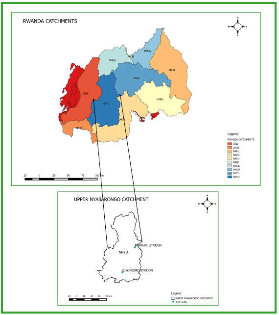
The upper Nyabarongo catchment has no dependency on any upstream catchments, Hence Waterflow and quality are defined within the catchment itself. The outflow of the catchment is at the confluence of the Mukungwa and Upper Nyabarongo Rivers where the Nyabarongo turns and takes a south easterly direction [16]. Upper Nyabarongo catchment has code of NNYU and it cover these districts: (Karongi, Ngororero, Rutsiro, Muhanga, Huye, Nyamagabe, Nyanza, Nyaruguru, Ruhango); its surface area is 3 348 Km2, Average rain fall which is equal 1365 mm, its sub-catchmdents are: NNYU- 1Mbirurume, NNYU-2 Mwogo, NNYU-3 Remainder; its Approx.Base flow (m3/s) equal to 34.2 and Approx Peak Flow(m3/s) are 207. The catchment is characterized by soil erosion from poor agricultural practices, illegal mining activities and deforestation, causing heavy siltation in Nyabarongo river and tributaries [17]. The major economic activities in Upper Nyabarongo are agriculture and livestock, hydropower, trade and mining (especially in the districts of Muhanga, Ngororero, Rutsiro, Ruhango, Nyamagabe, Huye and Nyanza) and small agro- industries.The catchment is also home to a number of coffee washing stations and tea factories.
Collection of Data
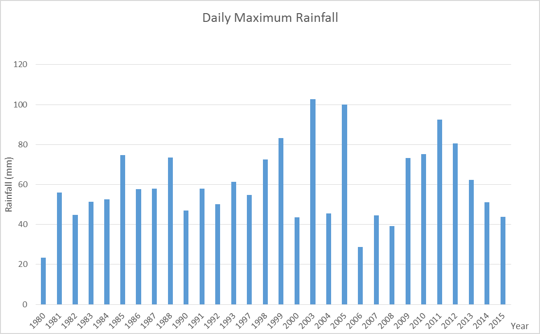
The data used in this work have been provided by the METEO-RWANDA which has the responsibility of measuring, analyzing and storing meteorological data and forecasting the weather in Rwanda. The data consisted of Daily maximum series (AMS) of rainfall depth over a period of thirty years for Gikongoro meteorological station (1980-2015) and also 36 for Byimana meteorological station (1980-2016)] for several laps of time: 10min, 20min, 30min, 60min, 120min, 180min, 360min, 720min, 144min. These are the weather station, in Upper Nyabarongo catchment that has relatively never stopped activity over 30 and 25 years for Gikongoro and Byimana, so that enough data were available to make a frequency analysis of extreme rainfalls. In This catchment however the latter has never worked in 1989 and since 1994 up to 1996 for Gikongoro station and (1994-1995); (2000-2009) for Byimana station. Data of those years METEO-RWANDA has not archived them properly due to lack of personnel and the aftermath of the Genocide of 1994. But there were some Daily AMS that has been digitized for the period 1997-2015 and 2010-2016; these have been included in this work. The gaps were filled by the information recorded in t meteorological books. These books are filled by the meteorological agents at the station; they note in, a lot of information about the daily weather among them, the rain depth given by a rain gauge after each day, the start time and end time of rainfall. Within our study area there are 2 stations used; Byimana meteorological station will be used by Ngororero, Muhanga, Ruhango and Karongi districts. However, Gikongoro station will be used by Nyamagabe, Nyanza, Huye and Nyaruguru districts in the NNYU.
Method of Deriving IDF Curves
For a deep analysis on IDF curves, different methods can be used. There are three basic distinct approaches while constructing IDF curves.
A first consists of direct estimation of IDF curves from annual maximum rainfall by the use of plotting position formula for return period expressed as T below the length of available record. This approach produces non-smooth curves, but in the few cases when a long continuous record is available [18]. This is a viable alternative. More often, long records are available only for daily rainfall. Then the empirical IDF values for d=1 day may be used to calibrate the IDF curves generated by alternative procedures or to constrain the dependence of id, T on T [19]. A second approach, mostly followed in practice involves using a parametric model for id, T dependence on d and it is based on the typical shape of empirical IDF curves and dependence on T generally relies on the fact that rainfall maxima are attracted to extreme-type distributions. A wise analysis of annual extremes helps to determine the parameters of the model using various criteria. E.g. moment matching, maximum likelihood, least squares [20].
The third approach is so complicated. It consists of fitting temporal rainfall to continuous rainfall records and then use the model to generate rainfall time-series through Monte Carlo simulations; see for example [21]. It is important to note that model based IDF curves are smoother than the empirical ones and have approximate validity also beyond the range of the historical record. The shape of IDF curves should not be associated with a specific assumption but all available data should be used in case needed. This conceptually more satisfactory approach is rarely followed in practice because of complexities of formulating rainfall models, estimating their parameters, and generating Monte Carlo samples. Research on the extreme precipitation events is currently expanding and it is hoped this approach could be made easier to use [22]. Achievements carried out in the field of pluviometry modelling use several models including selective models involving isolated events [23]. In this research, have been preferred to use the second approach so as to establish IDF relationship. The reason for the choice is that this method is simple and provides reliable results. The moment matching method will be used as the better method for determining the parameter of statistic. It has been used for IDF generation by a lot of hydrological and meteorological services in World, as the Canadian weather service, NWS National Weather Service (USA), United Kingdom, Nigeria and elsewhere [24, 25, 26, 27, 28, 29, 30].
of Table 1; sampled extreme rainfall depth, in mm are ordered in descendent order. In column four values are exceedance probabilities obtained with Gringorten formula. The reduced valuable u is computed using expression. In the last column of the Table 1 are given the expected values as were directed by generated by Gumbel distribution. The mean and standard deviation of the sample and the parameters of the distribution are given below:
| Year | X(Observed) | rank | p | u | X(Gumb) |
|---|---|---|---|---|---|
| 2003 | 102.6 | 1 | 0.018592 | 3.975639 | 119.9926 |
| 2005 | 100 | 2 | 0.051793 | 2.93403 | 101.8434 |
| 2011 | 92.4 | 3 | 0.084993 | 2.421099 | 92.90593 |
| 1999 | 83.3 | 4 | 0.118194 | 2.073196 | 86.84399 |
| 2012 | 80.5 | 5 | 0.151394 | 1.806909 | 82.20413 |
| 2010 | 75.2 | 6 | 0.184595 | 1.589291 | 78.4123 |
| 1985 | 74.8 | 7 | 0.217795 | 1.403892 | 75.18187 |
| 1988 | 73.5 | 8 | 0.250996 | 1.241291 | 72.34866 |
| 2009 | 73.3 | 9 | 0.284197 | 1.095568 | 69.80955 |
| 1998 | 72.6 | 10 | 0.317397 | 0.962748 | 67.49527 |
| 2013 | 62.2 | 11 | 0.350598 | 0.840018 | 65.35678 |
| 1993 | 61.3 | 12 | 0.383798 | 0.725297 | 63.35786 |
| 1987 | 58 | 13 | 0.416999 | 0.616991 | 61.4707 |
| 1991 | 57.9 | 14 | 0.450199 | 0.513831 | 59.67323 |
| 1986 | 57.8 | 15 | 0.4834 | 0.41478 | 57.94732 |
| 1981 | 56 | 16 | 0.5166 | 0.318951 | 56.27758 |
| 1997 | 54.8 | 17 | 0.549801 | 0.225565 | 54.6504 |
| 1984 | 52.6 | 18 | 0.583001 | 0.133906 | 53.05331 |
| 1983 | 51.4 | 19 | 0.616202 | 0.043285 | 51.47431 |
| 2014 | 51.1 | 20 | 0.649402 | -0.04699 | 49.90126 |
| 1992 | 50.1 | 21 | 0.682603 | -0.13767 | 48.32123 |
| 1990 | 46.9 | 22 | 0.715803 | -0.22959 | 46.7196 |
| 2004 | 45.6 | 23 | 0.749004 | -0.32376 | 45.07879 |
| 1982 | 44.7 | 24 | 0.782205 | -0.42147 | 43.37632 |
| 2007 | 44.5 | 25 | 0.815405 | -0.52449 | 41.58131 |
| 2015 | 43.8 | 26 | 0.848606 | -0.63545 | 39.6479 |
| 2000 | 43.6 | 27 | 0.881806 | -0.75867 | 37.50089 |
| 2008 | 39.2 | 28 | 0.915007 | -0.90227 | 34.9988 |
| 2006 | 28.8 | 29 | 0.948207 | -1.08536 | 31.80853 |
| 1980 | 23.4 | 30 | 0.981408 | -1.38254 | 26.63039 |
Table 1: Daily AMS Analysis for Gikongoro station.
O: Observed frequency; E: Expected frequency
NO years 0.167hr 0.33hr 0.5hr 1hr 2hr 3hr 6hr 12hr 24hr 1 1980 4.541952 5.68664 6.52238 8.198722 10.3059 11.78138 14.80935 18.61555 23.4 2 1981 10.86963 13.60905 15.6091 19.62087 24.6637 28.19476 35.44118 44.55004 56 3 1982 8.676294 10.86294 12.4594 15.66166 19.68692 22.50546 28.28966 35.56048 44.7 4 1983 9.976767 12.49117 14.3269 18.00916 22.63775 25.87876 32.52994 40.89058 51.4 5 1984 10.20969 12.78279 14.6614 18.42961 23.16626 26.48293 33.2894 41.84522 52.6 6 1985 14.51872 18.17781 20.8493 26.20788 32.94366 37.66014 47.3393 59.50613 74.8 7 1986 11.21901 14.04649 16.1108 20.25154 25.45646 29.10102 36.58037 45.98201 57.8 8 1987 11.25783 14.09509 16.1666 20.32162 25.54455 29.20171 36.70694 46.14112 58 9 1988 14.26639 17.86188 20.487 25.7524 32.37111 37.00562 46.51655 58.47193 73.5 10 1990 9.103315 11.39758 13.0726 16.43248 20.65585 23.61311 29.68199 37.31066 46.9 11 1991 11.23842 14.07079 16.1387 20.28658 25.5005 29.15136 36.64365 46.06156 57.9 12 1992 9.724437 12.17524 13.9646 17.55367 22.0652 25.22424 31.7072 39.85638 50.1 13 1993 11.89836 14.89705 17.0864 21.47785 26.99794 30.86319 38.79544 48.76639 61.3
| 14 | 1997 | 10.63671 | 13.31743 | 15.2746 | 19.20043 | 24.13519 | 27.59058 | 34.68173 | 43.5954 | 54.8 |
| 15 | 1998 | 14.0917 | 17.64317 | 20.2361 | 25.43706 | 31.97472 | 36.55249 | 45.94696 | 57.75595 | 72.6 |
| 16 | 1999 | 16.16857 | 20.24347 | 23.2186 | 29.18605 | 36.68725 | 41.9397 | 52.71876 | 66.26819 | 83.3 |
| 17 | 2030 | 8.462783 | 10.59562 | 12.1528 | 15.27625 | 19.20245 | 21.95163 | 27.59349 | 34.68539 | 43.6 |
| 18 | 2003 | 19.91472 | 24.93373 | 28.5981 | 35.94824 | 45.18742 | 51.65682 | 64.93331 | 81.62204 | 102.6 |
| 19 | 2004 | 8.850984 | 11.08166 | 12.7103 | 15.977 | 20.0833 | 22.95859 | 28.85925 | 36.27646 | 45.6 |
| 20 | 2005 | 19.41005 | 24.30188 | 27.8734 | 35.03727 | 44.04232 | 50.34778 | 63.28783 | 79.55365 | 100 |
| 21 | 2006 | 5.590095 | 6.998942 | 8.02755 | 10.09073 | 12.68419 | 14.50016 | 18.22689 | 22.91145 | 28.8 |
| 22 | 2007 | 8.637474 | 10.81434 | 12.4037 | 15.59159 | 19.59883 | 22.40476 | 28.16308 | 35.40137 | 44.5 |
| 23 | 2008 | 7.608741 | 9.526337 | 10.9264 | 13.73461 | 17.26459 | 19.73633 | 24.80883 | 31.18503 | 39.2 |
| 24 | 2009 | 14.22757 | 17.81328 | 20.4312 | 25.68232 | 32.28302 | 36.90492 | 46.38998 | 58.31282 | 73.3 |
| 25 | 2010 | 14.59636 | 18.27501 | 20.9608 | 26.34803 | 33.11982 | 37.86153 | 47.59245 | 59.82434 | 75.2 |
| 26 | 2011 | 17.93489 | 22.45494 | 25.7551 | 32.37444 | 40.6951 | 46.52135 | 58.47795 | 73.50757 | 92.4 |
| 27 | 2012 | 15.62509 | 19.56301 | 22.4381 | 28.205 | 35.45407 | 40.52996 | 50.9467 | 64.04069 | 80.5 |
| 28 | 2013 | 12.07305 | 15.11577 | 17.3373 | 21.79318 | 27.39432 | 31.31632 | 39.36503 | 49.48237 | 62.2 |
| 29 | 2014 | 9.918537 | 12.41826 | 14.2433 | 17.90405 | 22.50563 | 25.72771 | 32.34008 | 40.65191 | 51.1 |
| 30 | 2015 | 8.501603 | 10.64422 | 12.2086 | 15.34633 | 19.29054 | 22.05233 | 27.72007 | 34.8445 | 43.8 |
| Mean | 11.65833 | 14.59652 | 16.7417 | 21.04455 | 26.45329 | 30.24055 | 38.01278 | 47.78257 | 60.06333 | |
| DTDEV.S | 3.762131 | 4.710284 | 5.40254 | 6.791059 | 8.536452 | 9.758601 | 12.26669 | 15.4194 | 19.38239 |
Table 2: Shorter Duration Rainfalls Derived from Max.
| YEARS | %(Observed) | rank | p | to | X(Gumb) |
|---|---|---|---|---|---|
| 2012 | 91.7 | 1 | 0.02229299 | 3.7922314 | 114148327 |
| 1983 | 84.7 | 2 | 0.06210191 | 2.7470928 | 97.2894704 |
| 2016 | 82.9 | 3 | 0.10191083 | 2.23039546 | 88.9547611 |
| 1990 | 79 | 4 | Q14171975 | 1.87846445 | 83.2778542 |
| 1982 | 78.2 | 5 | Q18152866 | 1.60786466 | 78.9127136 |
| 2014 | 76.6 | 6 | 0.22133758 | 1.38558391 | 75.3273273 |
| 1987 | 72.8 | 7 | 0.2611465 | 1.19515971 | 72.25^^5 |
| 1988 | 66.8 | 8 | 0.30095541 | 1.02710846 | 69.5443539 |
| 1986 | 68 | 9 | 0.34076433 | 0.87545068 | 67.0385019 |
| 2011 | 68 | 10 | 0.38057325 | 0.73613647 | 64851261 |
| 1992 | 65.8 | 11 | 0.42038217 | 0.60626093 | 62.7562727 |
| 2013 | 63.9 | 12 | 0.46019108 | 0.48363198 | 60.7781772 |
| 1993 | 63.1 | 13 | 0.5 | 0.36651292 | 588863 |
| 1980 | 61.9 | 14 | 0.53980892 | 0.25345653 | 57.0652774 |
| 2010 | 61.7 | 15 | 0.57961783 | 0.143.13808 | 55.2865659 |
| 1984 | 61.4 | 16 | 0.61942675 | 0.03451214 | 53.5335427 |
| 1998 | 61.2 | 17 | 0.65923567 | -0.07377463 | 51.7867973 |
| 1985 | 57.4 | 18 | 0.69904459 | -0.1829823 | 50.025197 |
| 1981 | 52.6 | 19 | 0.7388535 | -0.29466295 | 48.2237056 |
| 1991 | 93.4 | 20 | 0.77866242 | -0.41032819 | 46.3498746 |
| 2015 | 48.2 | 21 | 0.81847134 | -0.53435173 | 44.3573488 |
| 1989 | 36.2 | 22 | 0.85828025 | -0.66982932 | 42.1719953 |
| 1999 | 31 | 23 | 0.89808917 | -0.82577814 | 39.65E4257 |
| 1997 | 28.6 | 24 | 0.93789809 | -1.02203342 | 36.4898767 |
| 1996 | 24.4 | 25 | 0.97770701 | -1.33591718 | 31.4275066 |
Table 3: Daily AMS analysis for BYIMANA Meteorological station.
Result and Discussion
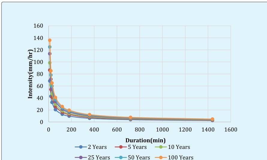
From the raw data, the maximum rainfall (P) and the statistical variables (average and standard deviation) for each duration (10, 20, 30, 60, 120, 180, 360, 720, 1440 min) were calculated. Various duration of rainfalls like 10, 20, 30, 60, 120, 180,360, 720 and1440 min were estimated from annual maximum 24 hours rainfall data using Indian Meteorological empirical reduction formula. These estimated various duration data were used in Gumbel’s Extreme Probability Method to determine rainfall (Pt) values and intensities (IT) for two meteorological stations. Rainfall frequency (Pt) values and intensities (IT) for different durations and return periods using Gumbel Method for Gikongoro station was computed. Similarly, for all other station, rainfall frequency (Pt) values and intensities (IT) for different durations and return periods using Gumbel Method was computed. Both Tables 4 and 6, it was found that intensity of rainfall decreases with increase in storm duration. Further, a rainfall of any given duration will have a larger intensity if its return period is large. After finding out the rainfall (Pt) values and intensities (IT) in Figure 5 and 6 Rainfall IDF curves are developed for two stations. Then finally for each station for each return period an equation has been developed, shown in Table 5 to table 7. It was found that the correlation coefficient for each equation is 1 which indicates a strong relationship in IDF equations.
| Return period | x | y | Equations | Correlation coefficient(R) |
| 2 | 309.3 | 0.67 | i=309.3(td)^{-0.67}$ | R=1 |
| 5 | 402.36 | 0.67 | i=402.36(td)^{-0.67}$ | R=1 |
| 10 | 464.12 | 0.67 | i=464.12(td)^{-0.67}$ | R=1 |
| 25 | 542 | 0.67 | i=542(td)^{-0.67}$ | R=1 |
| 50 | 599.75 | 0.67 | i=599.75(td)^{-0.67}$ | R=1 |
| 100 | 675.19 | 0.67 | i=657.19(td)^{-0.67}$ | R=1 |
Table 4: Rainfall IDF empirical equation for respective return period and their correlation coefficient, R for Gikongoro Table 4:
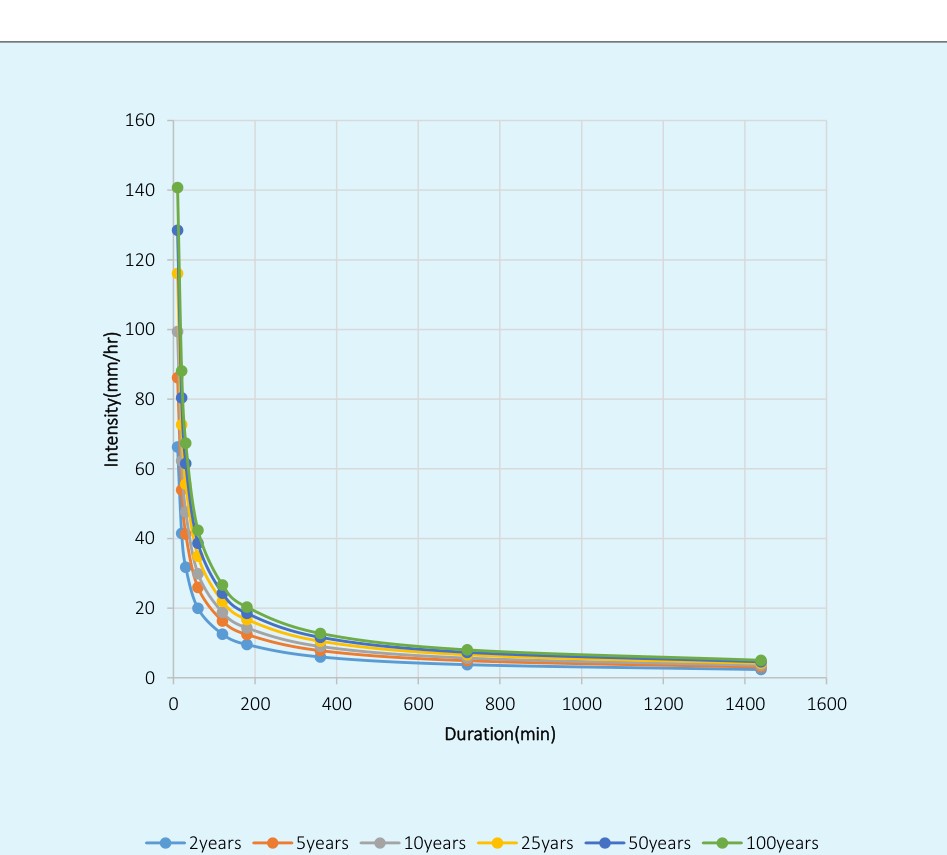
Figure 5: Rainfall IDF curve (Gikongoro station). To estimate the maximum rainfall intensity for different duration and return periods the following empirical equation is used. i = x * (td) -y Where, i = rainfall intensity in mm/hr., td = rainfall duration in minutes and x and y are the parameters to fit the IDF curve Least Square method is used to find parameters x and y for various return periods and the results are shown in table 14 and 16.
| 10min | 20min | 30min | |||||||||||||||
| Tr(Year) | MEAN | K | S | PT | I(mm/hr) | Tr(Year) | MEAN | K | S | PT | I(mm/hr) | Tr(Year) | MEAN | K | S | PT | I(mm/hr) |
| 2 | 11.658325 | -0.164 | 3.762131 | 11.04134 | 66.24801 | 2 | 14.59652 | -0.164 | 4.710284 | 13.82403 | 41.4721 | 2 | 16.74171 | -0.164 | 5.402535 | 15.85569 | 31.71139 |
| 5 | 11.658325 | 0.719 | 3.762131 | 14.3633 | 86.17978 | 5 | 14.59652 | 0.719 | 4.710284 | 17.98321 | 53.94964 | 5 | 16.74171 | 0.719 | 5.402535 | 20.62613 | 41.25227 |
| 10 | 11.658325 | 1.305 | 3.762131 | 16.56791 | 99.40744 | 10 | 14.59652 | 1.305 | 4.710284 | 20.74344 | 62.23032 | 10 | 16.74171 | 1.305 | 5.402535 | 23.79202 | 47.58404 |
| 25 | 11.658325 | 2.044 | 3.762131 | 19.34812 | 116.0887 | 25 | 14.59652 | 2.044 | 4.710284 | 24.22434 | 72.67302 | 25 | 16.74171 | 2.044 | 5.402535 | 27.78449 | 55.56899 |
| 50 | 11.658325 | 2.592 | 3.762131 | 21.40977 | 128.4586 | 50 | 14.59652 | 2.592 | 4.710284 | 26.80558 | 80.41673 | 50 | 16.74171 | 2.592 | 5.402535 | 30.74508 | 61.49016 |
| 100 | 11.658325 | 3.137 | 3.762131 | 23.46013 | 140.7608 | 100 | 14.59652 | 3.137 | 4.710284 | 29.37268 | 88.11805 | 100 | 16.74171 | 3.137 | 5.402535 | 33.68946 | 67.37893 |
| 60min | 120min | 180min | |||||||||||||||
| Tr(Year) | MEAN | K | S | PT | I(mm/hr) | Tr(Year) | MEAN | K | S | PT | I(mm/hr) | Tr(Year) | MEAN | K | S | PT | I(mm/hr) |
| 2 | 21.044554 | -0.164 | 6.791059 | 19.93082 | 19.93082 | 2 | 26.45329 | -0.164 | 8.536452 | 25.05331 | 12.52665 | 2 | 30.24055 | -0.164 | 9.758601 | 28.64014 | 9.546714 |
| 5 | 21.044554 | 0.719 | 6.791059 | 25.92733 | 25.92733 | 5 | 26.45329 | 0.719 | 8.536452 | 32.59099 | 16.2955 | 5 | 30.24055 | 0.719 | 9.758601 | 37.25699 | 12419 |
| 10 | 21.044554 | 1.305 | 6.791059 | 29.90689 | 29.90689 | 10 | 26.45329 | 1.305 | 8.536452 | 37.59336 | 18.79665 | 10 | 30.24055 | 1.305 | 9.758601 | 42.97553 | 14.32518 |
| 25 | 21.044554 | 2.044 | 6.791059 | 34.92548 | 34.92548 | 25 | 26.45329 | 2.044 | 8.536452 | 43.90179 | 21.9509 | 25 | 30.24055 | 2.044 | 9.758601 | 50.18713 | 16.72904 |
Table 5: Computed frequency rainfall (PT) values and intensities (IT) for different durations and return periods using Gumbel for
| 10min | 20min | 30min | |||||||||||||||
| Tr(Year) | MEAN | K | S | Pt(σ+K*S) | l(mm/hr) | Tr(Year) | MEAN(σ) | K | S | Pt(σ+K*S) | l(mm/hr) | Tr(Year) | MEAN(σ) | K | S | Pt(σ+K*S) | l(mm/hr) |
| 2 | 11.9449467 | -0.164 | 3.417313 | 11.3845074 | 68.3070444 | 2 | 14.9553776 | -0.164 | 4.27856339 | 14.2536932 | 42.7610796 | 2 | 17.1533079 | -0.164 | 4.90736625 | 16.3484998 | 32.6969997 |
| 5 | 11.9449467 | 0.719 | 3.417313 | 14.4019948 | 86.4119687 | 5 | 14.9553776 | 0.719 | 4.27856339 | 18.0316647 | 54.094994 | 5 | 17.1533079 | 0.719 | 4.90736625 | 20.6817042 | 41.3634085 |
| 10 | 11.9449467 | 1.305 | 3.417313 | 16.4045402 | 98.4272412 | 10 | 14.9553776 | 1.305 | 4.27856339 | 20.5389028 | 61.6167084 | 10 | 17.1533079 | 1.305 | 4.90736625 | 23.5574209 | 47.1148417 |
| 25 | 11.9449467 | 2.044 | 3.417313 | 18.9299345 | 113.579607 | 25 | 14.9553776 | 2.044 | 4.27856339 | 23.7007612 | 71.1022835 | 25 | 17.1533079 | 2.044 | 4.90736625 | 27.1839645 | 54.3679291 |
| 50 | 11.9449467 | 2.592 | 3.417313 | 20.802622 | 124.815732 | 50 | 14.9553776 | 2.592 | 4.27856339 | 26.0454139 | 78.1362417 | 50 | 17.1533079 | 2.592 | 4.90736625 | 29.8732012 | 59.7464025 |
| 100 | 11.9449467 | 3.137 | 3.417313 | 22.6650576 | 135.990346 | 100 | 14.9553776 | 3.137 | 4.27856339 | 28.3772309 | 85.1316928 | 100 | 17.1533079 | 3.137 | 4.90736625 | 32.5477158 | 65.0954317 |
| 60min | 120min | 180min | |||||||||||||||
| Tr(Year) | MEAN | K | S | Pt(σ+K*S) | l(mm/hr) | Tr(Year) | MEAN(σ) | K | S | Pt(σ+K*S) | l(mm/hr) | Tr(Year) | MEAN(σ) | K | S | Pt(σ+K*S) | l(mm/hr) |
| 2 | 21.5619375 | -0.164 | 6.16862501 | 20.550283 | 20.550283 | 2 | 27.1036438 | -0.164 | 7.75404414 | 25.8319805 | 12.9159903 | 2 | 30.9840223 | -0.164 | 8.86417629 | 29.53.2947 | 9084343245 |
| 5 | 21.5619375 | 0.719 | 6.16862501 | 25.9971788 | 25.9971788 | 5 | 27.1036438 | 0.719 | 7.75404414 | 32.6788015 | 16.3394008 | 5 | 30.9840223 | 0.719 | 8.86417629 | 37.357365 | 12.452455 |
Table 6: Computed frequency rainfall (PT) values and intensities (IT) for different durations and return periods using Gumbel for
| Return Period (Years) | X | Y | Equation (i=X*(td)-y) | Correlation coefficient | |||||||||
|---|---|---|---|---|---|---|---|---|---|---|---|---|---|
| 2 | 318.91 | -0.67 | i=318.91(td)-0.67 | R=1 | |||||||||
| 5 | 447.79 | -0.686 | i=403.44(td)-0.67 | R=1 | |||||||||
| 10 | 459.54 | -0.67 | i=459.54(td)-0.67 | R=1 | |||||||||
| 25 | 530.28 | -0.67 | i=530.28(td)-0.67 | R=1 | |||||||||
| 50 | 582.74 | -0.67 | i=582.74(td)-0.67 | R=1 | |||||||||
| 100 | 634.92 | -0.67 | i=634.92(td)-0.67 | R=1 |
Table 7: Rainfall IDF empirical equation for respective return period and their correlation coefficient, R for BYIMANA Table 7: R
Conclusion and Recommendations
This research presents some insight into the way in which the rainfall is estimated in Upper Nyabarongo catchment. The results obtained showed a good match between the rainfall intensity computed by the method used and the values estimated by the calibrated formula with a correlation coefficient of greater than 0.98. This indicated the goodness of fit of the formula to estimate IDF curves in the region of interest for durations varying from 10 to 1440 min and return periods from 2 to 100 years. They will be used in design of safe and economical drainage facilities and operation or maintenance of municipal water management infrastructures such as culverts, drain, sewers, conveyance systems, bridges, roads, etc.… for Upper Nyabarongo catchment and its environs. Further researches should be conducted all around the country (in the remaining catchments) because this research emphasized on the single central catchment only, this will lead to the generation of empirical equations of rainfall intensity which will be used in the hydraulic design of the conveyance structures in Rwanda [31, 32, 33, 34, 35, 36, 37].
References
-
Mbajiorgu CC, Okonkwo GI (2010) Rainfall Intensity- Duration-Frequency Analysis for Southeastern Nigeria. CIGR J 12(1): 22-30.
-
Dupont BS, Allen DL, Clark KD (2000) Tevision of the rainfall-intensity-duration curves for the common wealth of kentucky. Kentucky: kentucky transportation center.
-
Dupont BS, Allen DL, Clark KD (2000) Revision of the Rainfall-Intensity-Duration Curves for the Commonwealth of Kentucky. Kentucky transportation center, college of engineering, University of Kentucky Lexington, Kentucky, UDA. P.1-S.N.
-
Dupont BS, Allen DL, Clark KD (2000) Revision of lexington, kentucky: Kentucky transportation.
-
Midimar (2012) Identification of disaster high risk zones on floods and landslides. Kigali: S.N.
-
Van De Vyver H, Demaree GR (2010) Construction of intensity-duration-frequency (idf) curves for precipitation at lubumbashi, congo under the hypothesis of inadequate data. Hydrol Sci J 55(4): 555-564.
-
Kotei R, Kyei-Baffour N, Ofori E, Agyare WA (2013) Rainfall trend, changes and their socio-economic and ecological impacts on the sumampa catchment for the 1980-2019 period. Int J Eng Res Technol Ind 2(6): 578-590.
-
Meyer A (1928) Hydrology. 2nd (Edn.), In: John SM. Wlley & Sons, pp: 298.
-
Sherman CW (1932) Frequency and intensity of excessive rainfalls. Trans ASCE 95: 951-960.
-
Bernard M (1932) Formulas for Rainfall Intensities of Long Durations. Transact Ame Society Civil Engineers 96(1): 592-624.
-
Hershfield (1961) Technical Paper No. 40, Rainfall frequency atlas of the united states, United States: Luther H. Hodges, Secretary.
-
Frederick (1977) Five to 60¬minute precipitation frequency. Noaa technical memorandum, nws hydro¬35. Eastern and central United States: Silver Spring.
-
Oyebande L (1982) Deriving Rainfall-Intensity- Duration-Frequency Relationships and Estimates for regions with inadequate data. Hydrol Sci J Des Sci Hydrolog 27(3): 353-367.
-
Demarée Gr (2004) Intensity-Duration-Frequency (IDF) curves for yangambi, congo, based upon long- term highfrequency precipitation data set. pp: 12.
-
Veneziano D, Langousi A, Furcolo P (2006) Multi- Fractality And Rainfall Extremes: A Review. Water Resour Res 42(6).
-
(2011-2012) Consultancy services for development of rwanda national water resources master plan. S.L.: Rwanda Natural Resources Authority.
-
(2011) Rwanda launches upper nyabarongo catchment rehabilitation. S.L.: S.N.
-
Daniele Veneziano, Chiara L, Andreas L, Pierluigi FA (2007) Marginal Methods of IDF Estimation in scaling and non-scaling rainfall. Massachusetts, 02139 (Edn.), Department of civil and environmental engineering massachusetts institute of technology Cambridge, USA.
-
Koutsoyiannis D (2004) Statistics of extremes and estimation of extreme rainfall: 1. Theoretical Investigation. Hydrol Sci J 49(4): 590.
-
Veneziano D, Furcolo P (2002) Multi-Fractality of Rainfall and Scaling of Intensity-Duration- frequency curves. Water Resour Res 38(12): 42/1-42/12.
-
Chow VT. Main DR. Mays LW (1988) Applied hydrology (Mcgraw-hill series in water ressource and environmental engineering). S.L.: S.N.
-
Young BC, Mcenroe BM (2002) Precipitation frequency estimates for the kansas. Kansas, Lawrence : University of kansas.
-
Coles S (2001) An introduction to statistical modeling of extreme values. Springer series in statistics, London: S.N.
-
Law (1991) Quadratic Statistics for the Goodnessof- Fit. Ieee Trans Reliab 41: 118-123.
-
Rashid MM, Faruque SB, Alam JB (2012) Modelling of short duration rainfall intensity duration frequency (sdr-idf) equation for sylhet city in bangladesh. ARPN Journal of Science and Technology 2(2): 91-95.
-
Brain WM, Shapiro SS, Chen HJ (1981) A Comparative Study of Various Tests for Normality. J Ame Statistics Association 63(324): 1343-1372.
-
Bruce (2002) Validating A Relationship between Avalanche Runout Distance and Frequency. International Snow Science Workshop Grenoble.
-
Calvin RW (2004) An introduction to the environmental physics of soil, water and watersheds. Uk: S.N.
-
Catchment WN Rwanda launches upper nyabarongo catchment rehabilitation, S.L.: S.N.
-
Chin DA (2000) Water-Resources Engineering. Prentice Hall, New Jersey: S.N.
-
Chowdhury, Rezaul KA, Md JBD Alam P, Md A (2007) Short Duration Rainfall Estimation of Sylhet: IMD and USWB Method. J Ind Water Works Ass 39(4): 285- 292.
-
Gunes H (1997) Modified Goodness-of-fit, computational statistics and Data. pp: 63-77.
-
Munshi Rasel, Sayed MH (2015) Development of rainfall intensity duration frequency (r-idf) equations and curves for seven divisions in bangladesh. Int Jf Scient Eng Res 6(5) 96-101.
-
Zope PE, Eldho TI, Jothiprakash V (2016) Development of rainfall intensity duration frequency curves for mumbai city, India. J Water Resou Prot 8(7): 756-765.
-
Rambabu P, Prajwala G, Navyasri KVSN, Sitaram AI (2016) Development of intensity duration frequency curves for narsapur mandal, telangana state, India. Int J Res Eng Technol 5(6): 109-113.
-
Vyver H. Van de, Demaree GR (2013) Construction of Intensity-Duration-Frequency (IDF) curves for precipitation with annual maxima data in rwanda, Central Africa. Adv Geosci 35: 1-5.
-
Henze N (1990) Empirical–distribution–function goodness–of–fit tests for discrete. Canad J Statist 24(1): 81-93.
- Lessons to Learn: Trees are More than the Lungs of the World
- Community Forestry Enterprises as a Model for Sustainable Forest Development: The Case Of The "Baja Tarahumara" in Chihuahua, Mexico
- Ecological and Socio-Economic Impacts of Chromolaena odorata and Mesosphaerum suaveolens, Two Invasive Alien Species in Central and Southern Benin, West Africa
- Epigenetic Sustainability: Modeling the Human Factor as a Natural Resource through Science 4.0 and the NR3C1 Biological Pilot
- Growth-at-Risk: A Framework for Assessing Economic Vulnerability
- The Rural Territory as a Socioecological System for the Management of Public Policy for Sustainable Rural Development