Forecasting the Next Parkfield Mainshock on the San Andreas Fault (California)

Introduction

A recent experimental work Vasseur [1] on predicting the time of rock failure under stress provides evidence for a detectable preparatory phase to the sample failure, the accuracy of the forecast depending on the inter-flaw distance in the material that is being probed. Because a large earthquake is a macroscopic failure of a highly heterogeneous crust, we expect observable precursory phases to exist, and a suitable way to detect them may be through the study of the spatial-temporal patterns of seismicity. However, these patterns are all recognized ex-post and are far from clear in precisely indicating the time of failure of a crustal fault. Interesting examples are those occurring prior to the 2009 L’Aquila earthquake: from a textbook-case of dilatance-diffusion pattern recognized by Lucente [2] that was detected the last weeks of the seismic cycle, to a 7 days periodic occurrence of foreshocks detected a few months before the mainshock about 3 km away from the hypocenter of the latter [3].

We thought that discovering the existence of a clear preparatory phase before a significant earthquake would probably have been easier if we chose a mature, vertical, relatively isolated strike-slip fault, where moderate main shocks (M6) recur on the same asperity with a relative regularity. We thus chose the transitional stretch of the San Andreas Fault (SAF), which produced, between 1857 and 1966, six moderate events with similar sizes (M6) and features that ruptured the same asperity with very close recurrence time intervals. Based on the mainshocks’ recurrence time, Bakun & Lindh [4] expected the next Parkfield earthquake before 1993, when in fact it occurred in 2004.

The Parkfield segment is located between the SAF creeping section, to the NW, and the locked portion of the SAF, to the SE, where occurred the January 9, 1857 Fort Tejon earthquake M7.9, with epicenter between Parkfield and Cholame [5, 6]. The objective of this study is the detection of spatial-temporal patterns of the activity during the Parkfield multiple cycles, and to use them to forecast. Once a pattern is recognized, it could be used to retrospectively predict the 2004 earthquake, and similar patterns could be used to forecast future mainshocks.

Data

The seismic catalog studied here was downloaded in the temporal interval between 01/01/1973 and 27/01/2019 (see Figure 1) from the Northern California Earthquake Data Center [7].

Click to enlarge

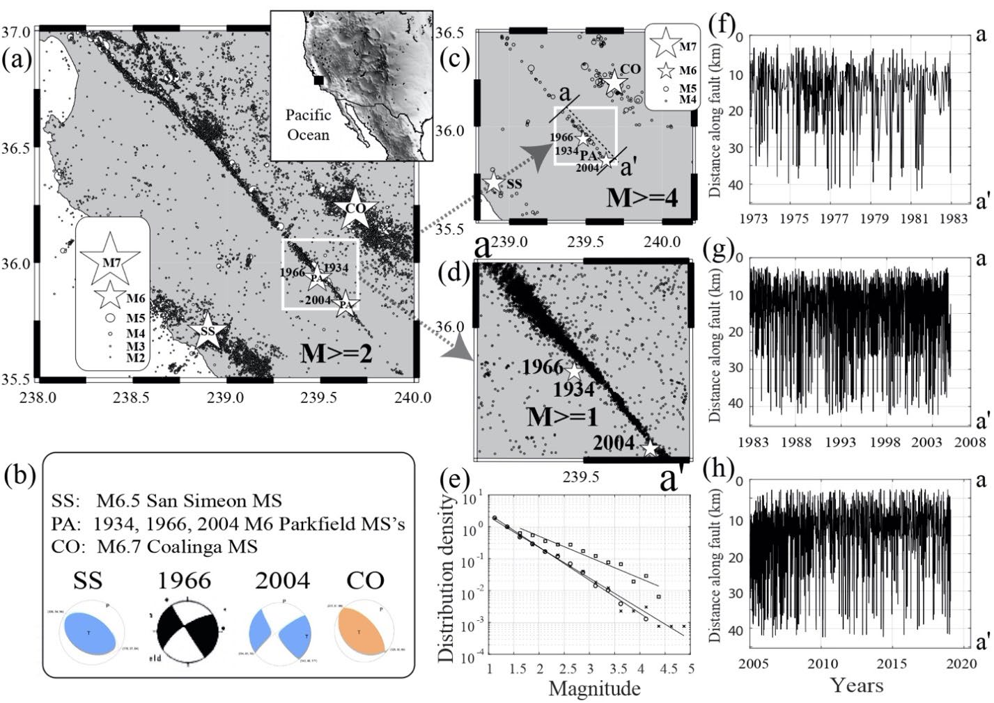
Figure 1: Catalog data plots. (a): Map of the region. Minimum magnitude is M1, but we plot the M2+ events (for magnitudes M ≥ 5 we use stars whose sizes scales with magnitude). The white square represents the region analysed in this study, includ- ing all significant seismicity occurring along the Parkfield segment of the SAF, and the epicenters of the 1934, 1966, and 2004 earthquakes. (b): Focal mechanisms of four major earthquakes: Coalinga (1983), San Simeon (1993), and Parkfield (1966, 2004). The catalog was taken from the California Integrates Seismic Network: Northern California Seismic System. (c): Earth- quakes from the catalog with M ≥ 4. (d): Zoom of the white square showing all M1+ events analyzed here. Stars indicate the locations of the 1934, 1966 and 2004 Parkfield mainshocks. (e): Magnitude of completeness analysis results of the earth- quakes plotted in (d): squares for interval 01/01/1973–31/12/1982; xs for interval 01/01/1983–31/12/2004; circles for interval 01/01/2005–27/01/2019. (f): Spatial center of daily seismic activity along the SAF fault in interval 01/01/1973– 31/12/1982. (g): as in (f), but for interval 01/01/1983–31/12/2004. (h): as in (f), but for interval 01/01/2005–27/01/2019.

Double differences locations are from Waldhauser [8, 9]. We considered a set of 9739 earthquakes from the region: -120.7W and -120.3W, 35.8N and 36.1N, 0 and 9 km depth, and in time interval between 01/01/1973 and 27/01/2019. The choice of our spatial window was suggested by the visual inspection of Figure 1(c) that shows that no notable earthquakes (M ≥ 4) occur outside such spatial window: to the NW the SAF is freely creeping, whereas to the SE the SAF is locked. In fact, since there is no notable seismicity SE of the 2004 mainshock, and there is a drastic reduction of seismicity NW of the NW corner of the white square, we decided to choose only events occurred within this square.

In what follows we analyse two temporal sequences: the spatial center of daily seismic activity along the fault Sebastiani [10] and the variance of the former within a moving time window for which we calculate an optimal width (see the Material and Methods section). Because the information that can be extracted from our catalog depends on its magnitude of completeness (MC), which has substantially decreased over time, we separately analyse three temporal intervals:

1. 01/01/1973 through 31/12/1982 (1256 events, MC1=1.5).
2. 01/01/1983 through 31/12/2004 (5300 events, MC2=1).
3. 01/01/2005 through 27/01/2019 (3183 events, MC3=MC2).

The last two intervals are naturally separated by the 2004 main shock, whereas the first one was independently analysed because its magnitude of completeness MC1 is largely higher than those, MC2 and MC3, of the other two intervals (see Figure 1e). No declustering was performed prior to computing completeness.

Material and Methods

For each of the three time intervals, we compute a spatial center of daily seismic activity c(t) along the axis, as introduced in Sebastiani [10]. The approach is based on the fact that the event spatial distribution is concentrated along an axis, i.e. the fault. In order to increase regularity, we apply Nadaraya-Watson kernel linear regression Eubanks [11]

to the sequence data ( ) ( ) ( ) { } 1 , 2 ,..., max y c c c t = to compute the estimated sequence ˆy . The kernel smoothing sequence parameter is estimated as proposed in Malagnini [12].

Based on the estimated sequence ˆy, we obtain a new sequence , ,....., 1 2 V V V = whose term Vi is the variance of the values { } 1 1 ˆ ˆ ,..., , T y y y i i i+ − + , where T is the length of the temporal window over which the variance is calculated. From the variance sequence V, we compute a set of local maxima (location, value): ( ) ( ) , , , ,...., 1 1 2 2 X M X M alternated to local minima ( ) ( ) , , , ,..., 1 1 2 2 x m x m as follows. The first maximum ( ) ,1 1 X M corresponds to the point of absolute maximum of V, while ( ) ,1 1 x m is the point of absolute minimum of ,...., 1 1 V VX .

The ( ) ,1 1 X M i i + + is the first point such that all values of V after

1 Xi+ are smaller than 1 Mi+ and the minimum value mi+1 of { } 1 ,..., i i V V X X + satisfies ( ) 2 1 1 i m M x i i < + + / is its location .

the set We then compute two straight lines. The first one is horizontal and corresponds to the best fit to the set of variance minima. No orientation constraint is imposed to the other line, which is obtained as best fit to the set of variance maxima. The forecast of the next mainshock is finally obtained as intersection between the two straight lines of above.

The value of the length T of the temporal window is found as follows. We compute the variance curve and the corresponding decreasing straight line for different values of T in a finite set of values. Then, the selected value of T is the one which minimizes the ratio of the mean squared error between the variance maxima and the corresponding best linear fit values to the variance of maxima.

After determining the points of variance maxima and minima, we compute the two spatial distributions along fault plane of the energy E, related to the magnitude M by E = 10[1.44M+5.24], of all events happened in a window corresponding to a point of either a maximum or a minimum, respectively Sebastiani [10]. To reduce the effect of spatial noise, the image representing the OCCO (opening-closing- closing-opening) operator of Mathematical Morphology Serra [13], Maragos & Schafer [14] is then computed from the support of the distributions.

Results

For each one of the three temporal intervals, we computed the sequence of the spatial center of daily seismic activity Sebastiani [10] (see the Material and Methods section), as shown in Figures 1f–1h. From the sequence of the spatial center of daily seismic activity, we calculate that of its variance on a moving time window (see Figure. 2(a)). In the three time intervals, the variance sequence show similar, non-symmetric oscillations, with a common minimum value. Moreover, the three sub-sequences have triangular envelopes, in which peaks linearly grow with time over a period of 6-8 years, reach a global maximum, then linearly decrease over a period of 13-17 years. The increasing phases for different cycles have similar slopes, and the same is true for the decreasing phases, suggesting that the same mechanism is acting in all cycles.

For the 1984–2004 time interval, when considering data up to 100 days before mainshock, its occurrence coincides with the interception of the horizontal line best fitting the variance sequence minima and the best linear fit to the peak values of decreasing amplitude, starting from the largest one. Based on this observation, we decided to empirically choose it as a retrospective forecast of the 2004 earthquake (see the Material and Methods section). We note that the amplitude of the forecast error is linearly related to the time separation between the end of data used for forecasting and the actual occurrence of the mainshock (see Figure 2b). Finally, in case of the third time interval (01/01/2005–27/01/2019), we produce a forecast for the next mainshock about 5.42 years since the end of the time interval (early June 2024).

Click to enlarge

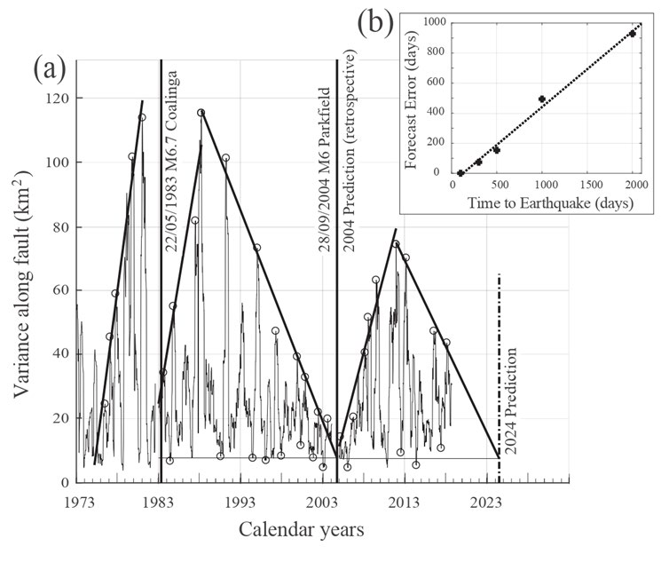
Figure 2: Variance analysis. (a): Variance of the spatial center of daily seismic activity along the SAF fault calculated on a mov- ing time window, for whose length an optimal value was found (see the Material and Methods section), between 01/01/1973 and 27/01/2019. The analysis has been carried out using three different temporal intervals: i) between 01/01/1973 and 31/12/1982; ii) between 01/01/1983 and 20/06/2004, i.e. 100 days before the M6 mainshock; iii) between 01/01/2005 and 27/01/2019. Indicated is the occurrence of the 02/05/1983 Coalinga earthquake (vertical red line), that caused an abortion of the Parkfield seismic cycle initiated in 1966. The M6 2004 Parkfield mainshock (vertical red line) coincides with our retro- spective forecast. Dashed-dotted red line indicates our forecast for the next mainshock. (b): Estimated forecast time error, as a function of time from the last data point used for forecasting to the actual occurrence of the 2004 main shock.

About the periodicities appearing on the variance time sequences of Figure 2(a), we analyse the 1983–2004 time interval, where a complete decreasing phase is present. The estimated period of a damped sinusoid model was 1113 days, as already observed on different phenomena in the same area [15, 16], thought to be related to pore pressure variations on the SAF [17].

Peak amplitudes of the variance time sequences yield information about the dimension of the patch during a specific temporal interval. For example, the largest peak of Figure 2(a), corresponds to a size a bit larger than 50 km2, whereas the value corresponding to the beginning of 2003, corresponds to a size a bit smaller than 10 km2. It is very interesting to see that the minima of the variance curve are fairly constant throughout the seismic cycle (a size of about 3 km2).

Click to enlarge

Figure 3: Energy spatial distribution. Support of the energy spatial distribution of events belonging to windows corresponding to (a): the variance minima of Figure 2(a) for the temporal interval 01/01/1983–20/06/2004, i.e. 100 days before 2004 mainshock; (b): as in A, but the variance maxima; (c),(d): as in (a) and (b), but for the temporal interval 01/01/2005– 27/01/2019. The bottom- right star in each cross-section corresponds to the hypocenter of the 2004 Parkfield earthquake. The curves roughly indicate the level contour corresponding to 20% of maximum coseismic slip of the 2004 Parkfield main shock, as inverted by Murray and Langbein [18]. Horizontal and vertical axes correspond to event distance along fault and depth, respectively.

The supports (in a mathematical sense) on the fault plane of the distributions of the total energy released by events belonging to windows of variance maxima and minima, are shown in Figure 3. Mathematical Morphology Serra [13] Maragos & Schafer [14] is applied to the supports to produce the images shown. We see that for both seismic cycles, maxima and minima of Figure 2(a) are related to seismic energy radiated by the same patch of the SAF, adjacent to the main asperity, to the NW. Moreover, there exist strong similarities between the portions of fault surface activated during the variance fluctuations of different seismic cycles.

Discussion

Below, we first summarize and then describe the six main features of the triangular pattern shown in Figure 2a: 1. The increasing phase (repeated three times during the studied time period with virtually the same slope).

2. The decreasing phase (repeated twice with virtually the same slope). 3. The periodicity. 4. Common value of the variance at the minima. 5. Resetting the process by the Coalinga earthquake. 6. The occurrence of a mainshock at the end of the decreasing phase.

1) The Increasing Phase We assume that the portion of the SAF that dominates the variance produces a relatively weak coupling through the presence of a multitude of microasperities like the ones where the repeating earthquakes occur. At the beginning of a seismic cycle, the amount of surface area that is weakly coupled along the SAF is very small and it grows over time as the fault heals. This happens in a portion of the fault that is continuously creeping. Correspondingly, the peaks of the variance sequence grow. As long as this process is able to sustain part of the stress acting on the adjacent locked asperity, failure is delayed. The linear increase in the peak amplitudes of the variance function over time indicates a linear increase in the weakly coupled fault surface.

2) The Decreasing Phase After a while into the seismic cycle, the surface of the weakly coupled fault patch reaches a maximum and starts decreasing. That is, the area of (weak) coupling starts getting eroded away, like in the case of the Tohoku-Oki giant earthquake of 2011. As the stress-driven erosion of the stress shield proceeds, more and more stress is transferred onto the adjacent seismogenic asperity, until failure occurs. Again, the linear decrease in the peak amplitudes suggests that the surface of the weakly coupled fault patch is eroded linearly over time.

3) The Periodicity The 3.05-year periodic behavior illustrated in Figure 2(a) seems pretty close to the 2-2.5-year period one found by Turner [16] (see their Figures 3 and 8). This is consistent with similar results observed by Malagnini [12] on seismic attenuation in the same area (see their Figure 2). Here, we make the hypothesis that these three 2-3 years periodic patterns are related to the 2.5 year periodic variations of the hydrostatic load induced by drought- wet cycles (see Figure 4 from: https://pangea.stanford. edu/news/california-drought-exceptional). We notice that Johnson [15] demonstrated how important is the role of the hydrostatic load in the stress modulation across the SAF at Parkfield. Finally, Malagnini and Parsons [19] suggested that the variations in (normal) stress around the SAF at Parkfield induce a variability in permeability and thus in the seismic attenuation of Figure 2 of Malagnini [12]. We think that the same stress variability induced by the varying hydrostatic load produces a clamping-unclamping cycle that alternatively increases and decreases the coupling of the SAF. Such variations may be of special importance on the transitional segment of the SAF, because it is a region where the fault is weakly engaged, and the variations in normal stress may produce variations in coupling that, however small, are substantial for the patch of the SAF that dominates the variance, and can be detected by our method. This could explain the periodic behavior of the variance sequence.

4) Common Variance Value of the Minima Minima of the spatial variance function are expected to be attained at clamping minima, as they are modulated by the hydrologic load (effective normal stress minima). If our interpretation is meaningful, the common-level variance minima represent indirect measurements of clamping min- ima, and are explained by the fact that the unlocked portion of the transitional segment of the SAF keeps moving while the engagement of the two sides of the fault cannot get any lower. In our model, if the engagement of the stress shield is minimum, its spatial extent is also expected to be small.

5) Resetting the Process by the Coalinga Earthquake Based on the available literature (e.g., Toda and Stein [20], see their Figure 5), it looks that the large drop in spatial variance corresponds to a drop in the Coulomb stress induced by the mainshock. The Coalinga Coulomb stress release thus caused a reset of the variance function to a “global” minimum. The mechanism is that of fault unclamping.

6) The Occurrence of a Mainshock Finally, a mainshock is expected to occur around a minimum of the effective normal stress, if no other stress perturbations are present, that is, around a variance minimum. The variance analysis of Figure 2(a) shows that, unlike the current seismic cycle, the previous one was abruptly aborted around 1983 and immediately resumed. This is consistent with the shear and Coulomb stress transfer from the 02/05/1983 M6.5 Coalinga earthquake [21], and from the 11 June and 22/07/1983 M6 Nuñez earthquakes [22, 23]. Due to the Coulomb stress transfer from these earthquakes, variance peak amplitudes drop close to their background level (Figure 2a), indicating an abrupt and substantial stress release affecting the Parkfield asperity [20]. We notice that between the Coalinga reset of the growth/erosion cycle, in 1983, and the occurrence of the 2004 earthquake elapsed a bit more than 21 years, a number very close to the regular time length of the seismic cycle at Parkfield [4].

A similar abortion mechanism could be related to the pattern of the initial part of the variance sequence (1973– 1975); in fact, a starting value of about 25 km2, is large enough to be compatible with a growing phase started at the occurrence of the M6 1966 Parkfield mainshock. However, no notable earthquakes occurred in the area considered between 1973 and 1976, indicating that the activation and growth of the active patch may be subjected to other phenomena, like a acceleration/deceleration of the SAF [16]. We notice that without the two abortions, whose lengths can be estimated on Figure 2a, the 2004 mainshock would have happened much earlier, around 1992, in agreement with the main statement that the earthquake was expected to occur before 1993 in the well-known paper by Bakun and Lindh [4]. Interestingly, unrelated to the former discussion, and differently from the clear signal on the seismic attenuation documented by Malagnini [12], no apparent effects on the variance curves are seen at the time of occurrence of the San Simeon earthquake, even though it pushed the Parkfield segment closer to failure [24]. Despite all the described complications, our forecast is based on simple observations, and we expect the next Parkfield main shock to occur in mid- 2024. The increasing (decreasing) trend of the local maxima of the spatial variance of the center of seismicity implies a growth (reduction) of the activated area of the fault. We envision the active patch adjacent to the Parkfield asperity (highlighted in Figure 3) as a dense set of micro asperities embedded in a velocity-strengthening matrix. Differently from the Japanese megathrust [25, 26], the eroded portion of the coupled area of the SAF at Parkfield did not participate to the 2004 rupture [18]. On the contrary, in the model in Mavrommatis [25], dynamic rupture propagation is still possible after erosion due to dynamic weakening. Our hypothesis is that the growth of the activated area is simply due to increasing frictional engagement, whereas the decreasing phase represents the erosion of a coupled portion of the fault area, with consequent stress transfer onto the adjacent asperity. From Figure 2(a), we see that the stable coupled area is eroded linearly throughout the interseismic period. The model in Mavrommatis [25] predicts almost linear asperity erosion in the case when the fault surface is laterally homogeneous.

Conclusions and Final Recommendations

An accurate retrospective forecast of the 2004 M6 Parkfield main shock, as well as the one of the next Parkfield main shock in mid-2024 are obtained here by the recognition of a pattern for the temporal changes of the fluctuations of a quantity relevant to describe the state of the system under study. Future research must be aimed at applying our approach extensively, to faults of increasing geometric complexities, starting in tectonic environments similar to the one investigated here (isolated strike-slip faults, purely transcurrent, transpressional, and transtensional crustal structures), continuing with large compressional seismogenic features, and finally in complex extensional fault systems like the ones that dominate the tectonics of the Apennines.

Data and Resources

The earthquake catalog used in this study was obtained from the Northern California Earthquake Data Center (NCEDC, https://www.ncedc.org, last access July 2019). Data are available at the Northern California Earthquake Data Center (see reference NCED, 2014).

Acknowledgements

The authors are thankful to the anonymous reviewer for the very useful comments and suggestions and to Ilaria Spassiani for critical reading of the manuscript and the help regarding manuscript revision. This work was partially supported by funding from Istituto Nazionale di Geofisica e Vulcanologia, Sezione di Roma 1, Italy.