Comparison Study between Different Methods Used in the Estimation of Reserves in well F-12 of Volve Field
The present paper deliberates a comparison study between volumetric and material balance methods used in the estimation of reserves in well F-12 of Volve field. Based on PVT and petrophysical data, the estimation of reserves is done by using volumetric method with Excel software. The material balance method is applied on the PVT data, tank data and production history data to provide estimation by using MBAL software. The volumetric method gives estimated oil in place of about 67,639,727.94 Sm3 and so the reserve is equal to 36,525,453.09 S m3. While the stock tank original oil in place (STOIP) generated from MBAL software is 19,607,700 Sm3 and so the reserve is estimated to 10,584,378 Sm3. The volumetric method is less accurate than material balance method because it is based on the assumption that the reservoir is static and homogeneous. This is the reason why volumetric method provides an overestimated reserve. So, the material balance method seems to be the best method because of the amount and the type of production data used.
Introduction
Among the many varied and multidisciplinary tasks of petroleum engineers undertake in the practice of their profession, none are individually more important than the estimation and classification of oil and gas reserves [1, 2, 3]. To estimate reserves, the petroleum engineers must also use an impressive array of more conventional engineering and mathematical tools, often including probability theory [4, 5, 6, 7, 8]. Reserves estimates form the basis for most development and operational decisions and are of critical importance in financing and other commercial arrangements that allows oil and gas developments to proceed in an orderly and efficient manner [9, 10, 11].
The role of reserves estimates in operational, financial, and policy decisions emphasizes the need for the estimates to be as accurate and current as possible. The methods used to estimate reserves and the accuracy of the result depend on the type, amount and the quality of geologic and engineering data available The different methods used to estimate reserves may be applied to be connected or to be compared together to provide a possible reliable estimation of the property.
Volve is shallow water (water depth is about 80 m) oil field discovered at 1993, located in the central part of the north sea (norwegian continental shelf), 200 kilometres west of Stavanger at the southern end of the Norwegian sector [12]. Volve produced oil (Block 15/9) from middle Jurassic sandstones of the Hugin formation. Elaborating a good economic evaluation is still considered to be vital practise for the success of any hydrocarbon field development and planning. Thus, to make a good economic evaluation, it is important to estimate reserves as accurate as possible, to evaluate the economic rentability of a reservoir. Hence, the aim of this paper is to evaluate the best method that can be used to estimate reserves with the maximum reliability. To accomplish the study, the main objective is to estimate the reserve of field X by using volumetric and material balance methods. The paper is structured in three sections: the section 1 is the introduction. The section 2 concerns the presentation of data, tools and methods used to achieve all the objectives. The section 3 is worried about results, following by discussion. The last section is the conclusion.
Methodology and Data Analysis
The Volve field was established with a jack up processing and drilling facility. This field started well drilling at 2007 with a life of expectancy for about 3-5 years. Volve produced with a peak rate of about 56,000 barrels per day, with a recovery rate of 54% of reserve estimates, it was shut down in September 2016 after field operation for over 8 years. The reservoir is formed as a small dome-shaped structure and believed to be formed due to the downfall of contiguous salt ridges for the period of the jurassic [12]. Faults as a consequence of salt tectonics are the dominant structure in Volve field. The western part of the structure is heavily faulted, mostly influenced by regional extension and communication across tain. The reservoir is located at a depth of 2750-3120 m True vertical depth subsea and about 20 m thick on the crest that ultimately reaches up to 100 m on the flanks of the structure. The field’s oil production came from the Hugin Formation, relatively pure sandstone of Middle Jurassic age. The wells on the field tested the sandstone reservoir at a depth of 2,700 m to 3,100 m. The severely faulted western area of the structure has high uncertainty as to pressure communication across faults. According to the report from the Norwegian Petroleum Directorate (NPD), the field is estimated to hold a recoverable reserve of 78.6 million barrels of oil and 1.5 billion cubic meters of gas. The field came on stream at 2008 and was decommissioned in September 2016 after 8.5 years in operation, more than double the planned productive life’s plan. The field was initially developed with a production life’s plan of three to five years of operation. However, the production Well 15/9-F11-A led to the discovery of untested reserves on the field, which leads to an increase of the recoverable reserves by 12%. The wells 15/9-F-15 A, 15/9-F-10, 15/9-F-11 T2 and 15/9- F-5 were drilled till the Triassic top (average vertical drilled depth 3500 m) in a water depth of about 80 m. Wire line suite available from the wells includes Gamma-ray, resistivity, sonic and density logs. Well reference section (Norwegian well 15/9-2 (STATOIL) from 3483 m to 3657 m, coord n58°25’34.06’’, E01°42’28.2’’ [13]. The formation consists of light brown to yellow, very fine to medium grained sandstones. Occasional coarse grained layers are found. The sandstones have fair sorting, and the grains are subangular to subarrounded. Shale and silstone partings are common. Carbonaceous material and coal fragments are abundant. Occasional thin coal beds can be observed. The sandstones are often bioturbated, but cross bedding can sometimes be observed. The sandstones are often calcareous and glaucotinic.
Equinor, the operator of Volve field have released all subsurface and production data set from the field. Three types of data in Volve field are used the PVT data, flash input data on fluid properties and production data. The PVT samples or data sets represent the actual fluid compositions and that reliable and representative laboratory procedures have been used. Notably, the vast majority of material balances assume that differential depletion data represent reservoir flow and that separator flash data may be used to correct for the wellbore transition to surface conditions. The PVT data and production data are presented in Tables 1 and 2, respectively.
| Pressure | Gas Oil Ratio | Oil FVF | Oil Viscosity | Gas FVF | Gas Viscosity |
|---|---|---|---|---|---|
| 250 | 143.5 | 1.48274 | 0.502 | 0.00487 | 0.27202 |
| 268.5 | 143.5 | 1.47728 | 0.519 | 0.004624 | 0.029292 |
| 300 | 143.5 | 1.4686 | 0.546 | 0.004302 | 0.031551 |
| 350 | 143.5 | 1.45623 | 0.589 | 0.003929 | 0.034856 |
| 400 | 143.5 | 1.44528 | 0.631 | 0 | 0 |
| 450 | 143.5 | 1.43549 | 0.673 | 0 | 0 |
| 500 | 143.5 | 1.41867 | 0.714 | 0 | 0 |
| 550 | 143.5 | 1.41136 | 0.754 | 0 | 0 |
| 600 | 143.5 | 1.40466 | 0.793 | 0 | 0 |
| 650 | 143.5 | 0 | 0.832 | 0 | 0 |
| Reservoirs Parameters | Volumetric Method | Material Balance Method | Reservoirs Parameters | Volumetric Method | Material Balance Method |
| Aquifer model | - | Small pot | Formation gor (sm3/ sm3) | - | 825 |
| Temperature (0C) | - | 110 | Oil gravity (API) | - | 29 |
| Initial Pressure (BarA) | - | 310.84 | Gas gravity (sp.gravity) | - | 0.88 |
| Porosity | 0.2213 | 0.2213 | Water salinity (ppm) | - | 151200 |
| Connate-water saturation (%) | 0.2 | 0.2 | Thickness (m) | 25 | - |
| Water compressibillity | 2.16E-06 | Area (km2) | 6 | - | |
| Relative permeability Residual Saturation | Krw=0.23 Kro=0 Krg=0 | Oil FVF (scf/STB) | 1.37 | - |
Table 1: PVT data.
| Volumetric Method | Material Balance Method | Reservoirs Parameters | Volumetric Method | Material Balance Method | |
|---|---|---|---|---|---|
| Aquifer model | - | Small pot | Formation gor (sm3/ sm3) | - | 825 |
| Temperature (0℃) | - | 110 | Oil gravity (API) | - | 29 |
| Initial Pressure (BarA) | - | 310.84 | Gas gravity (sp.gravity) | - | 0.88 |
| Porosity | 0.2213 | 0.2213 | Water salinity (ppm) | - | 151200 |
| Connate-water saturation (%) | 0.2 | 0.2 | Thickness (m) | 25 | - |
| Water compressibility | 2.16e-6 | Area (km2) | 6 | - | |
| Relative permeability Residual Saturation | Krw=0.23 Kro=0 Krg=0 | Oil FVF (scf/STB) | 1.37 | - |
Table 2: Summary of reservoir parameters.
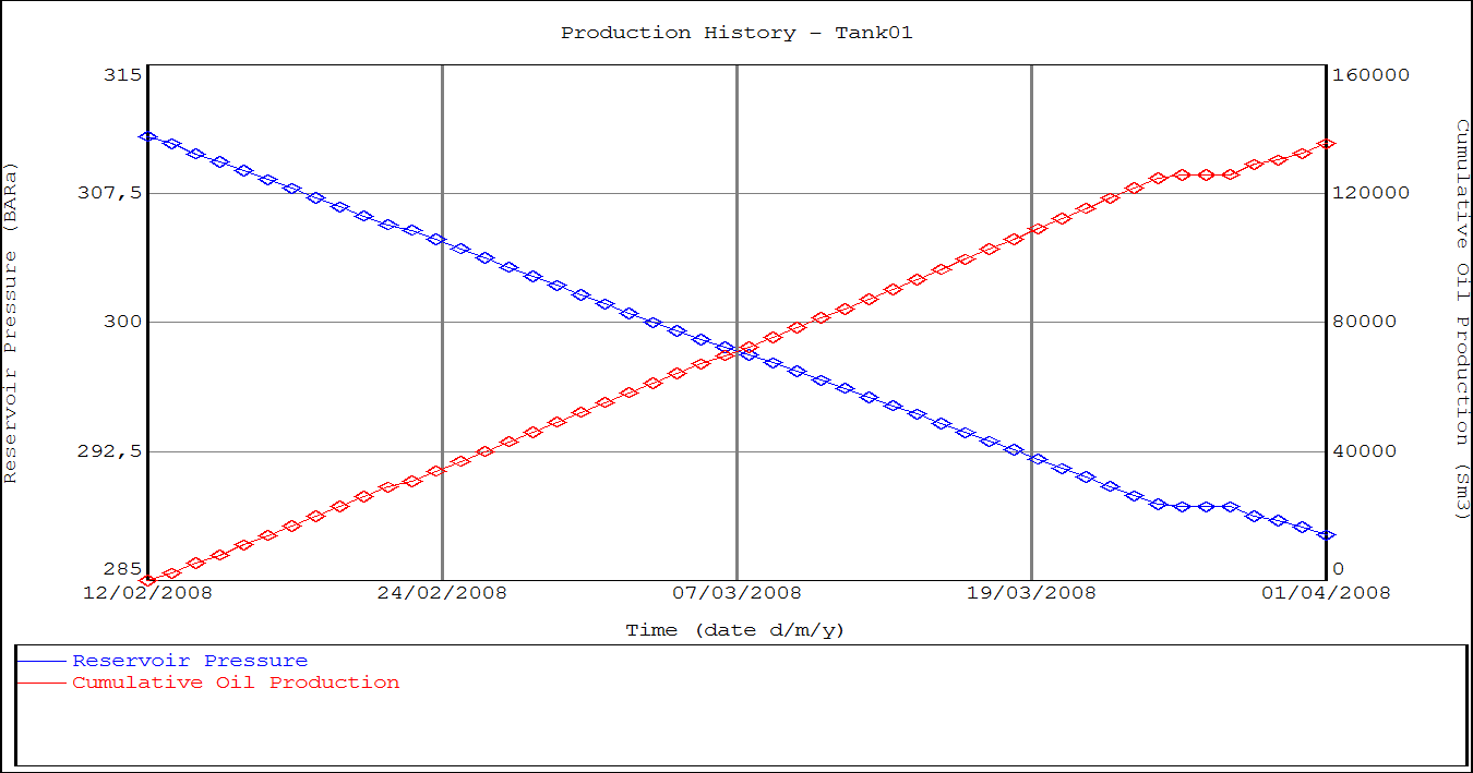
All production data should be recorded with respect to the same time period. If possible, gas-cap and solution-gas production record should be maintained separately. The production history of field X is presented in Figure 1.
The oil in place is determined by the volumetric method by using data generated from geological and petrophysical evaluation (area extent, formation sand thickness, porosity and saturation etc.) and computing the initial oil in place from the general formula:
( ) 1- , Ao Ho Sw Ni Boi
$$ i = \frac {\varphi * A o * H o * \left(\right)}{B o i} $$
(1) where Ni is oil initially in place, STB, is average porosity in the zone, fraction, Ao is area of the oil zone in acres, Ho is average oil thickness zone in feet, Sw is water saturation (fraction) and Boi is average initial formation volume factor in RB/STB. The equation of the material balance method was developed by Schilthius which equates the cumulative observed production (expressed as underground withdrawal) to the expansion of the fluid in the reservoir resulting from finite pressure drop which is the governing principle for the MBAL software. By using the material balance method, the Volume of oil in place is given by ( ) ( ) ( ) - - - , Np Bt Rs Rsi Bg We WpBw N S B B B mB B m B S $$ V = \frac {N p \left(B t + \left(R s - R s i\right) B g\right) - \left(W e - W p B w\right)}{B _ {t -} B _ {t i} + m B _ {t i} \frac {B _ {g}}{B _ {g i}} - 1 + B _ {t i} \left(1 + m\right) \left[ \frac {S _ {w i C _ {w} + C f}}{1 - S _ {w i}} \right]}, \tag { \textcircled{1} } $$ (2) ( ) - w wiC Cf g t ti ti ti gi wi + -1 1 1- where Bti is the total formation volume factor (bbl/STB); Cf is the formation compressiblity (psi-1); Cw is the water compressiblity (psi-1); Sw I the initial water saturation (%); M is the ratio of gas cap volume to oil volume (bbl/bbl); Bt is the total formation volume factor (bbl/STB); Bo is the oil formation volume factor at reservoir pressure (bbl/STB); Rsi is the gas solubility at initial pressure (scf/ STB), Rs is the gas solubility (scf/STB); Bg is the gas formation volume factor at reservoir pressure (bbl/STB), We is the cumulative water influx (bbl); Wp is the cumulative water produced (STB); and Bw is the water formation volume factor (bbl/STB). The various stages involved in the development of the model for the estimation of in place volume by using the material balance method include: PVT data, initial reservoir pressure, reservoir average pressure history, production history and all available reservoir and aquifer parameters.
Results and Discussions
The results obtained from the volumetric method calculations by using Excel software and simulations by using MBAL software are presented and discussed in this section.
For estimating reserves through the volumetric methods, the formula is integrated in Excel software following by data available. The estimation of well F-12 of Volve field reserve by using the volumetric method is presented in Table 3.
| Petrophysical data | Value | units |
|---|---|---|
| Thickness | 25 | m |
| Oil FVF | 1.37 | Scf/STB |
| Water Saturation | 20 | % |
| Porosity | 22.13 | % |
| Area | 6 | Km2 |
| Result | 67,639,727.94 | Sm3 |
Table 3: Volumetric method calculations on Excel software.
It is important to notice that these reservoir data are supposed constant when they are applied by volumetric method. The history matching is used to determine and identify sources of reservoir energy and their magnitude, the value of original oil in place, original gas in place, aquifer type and strength etc. The history matching in material balance method is the effective way to determine the aquifer model that best fits the observed data. Two different types of histories matching are used: Analytical and graphical methods. The analytical plot of reservoir versus cumulative oil production before and after regression is presented in Figure 2.
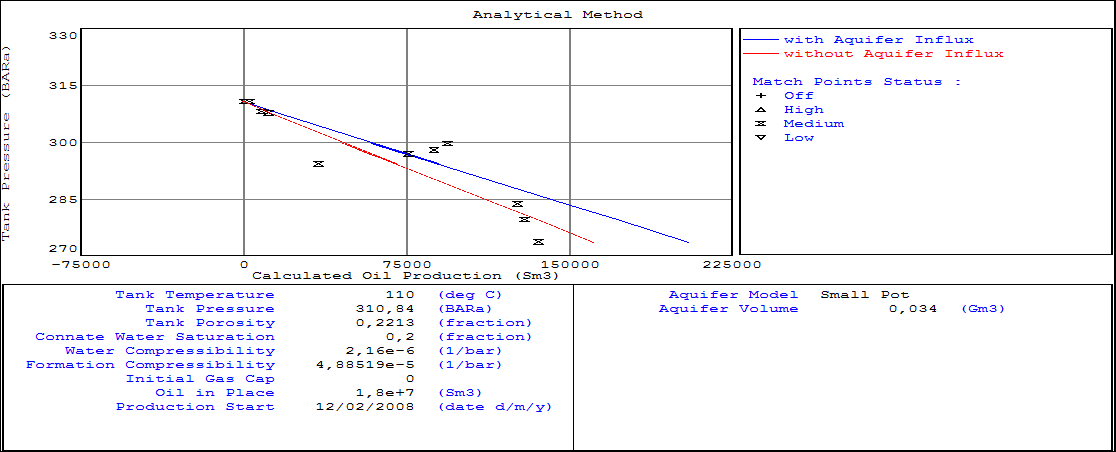
From Figure 2, it is observed that with the current aquifer model, the model was predicting the cumulative oil production higher than those observed without considering water influx initially when there is uncertainty of possible energy system. Plot shows considerable deviation between history matching data and history matched simulation model result. The red line shows the simulation model without aquifer strength while the blue line shows the simulated model with aquifer strength. It is important to notice that regression played a constructive role for eliminating the deviation between the simulated model and historical behavior in terms of production and pressure data [14, 15]. The analytical plot of reservoir pressure versus cumulative oil production before and after regression is presented in Figure 3.
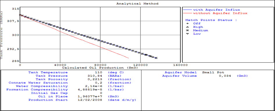
Figure 3 shows considerable deviation between history matching data and history matched simulation model result. The red line shows the simulation model without aquifer strength while the blue line shows the simulated model with aquifer strength. Basic graphical method for oil reservoir is given by $$ F = N E _ {t} + W _ {e}. \tag {3} $$ where F is the underground withdrawal, Et is the expansion of oil, N is the estimated STOIIP, and We is the cumulative water influx (in bbl). By rearranging equation (2), this expression is obtained:
$$ \frac {F - W _ {e}}{E t} = N. $$
(4) The parameter (F-/) versus F is plotted in Figure 4.
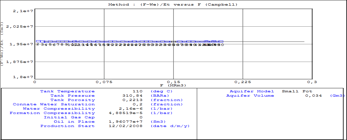
It is clearly seen in Figure 3 that the history points deviate from the horizontal. It indicates that the model is not able to predict the response as seen from the reservoir. For such reasons, building a correct aquifer model to match the production/ pressure data of the reservoir is always done on a ‘’ try and see’’ basis and even when a satisfactory model is achieved it is seldom. The parameter (F/We) versus (Et) is plotted in Figure 4 to obtain the ‘’N’’ value which is the estimated STOIP.
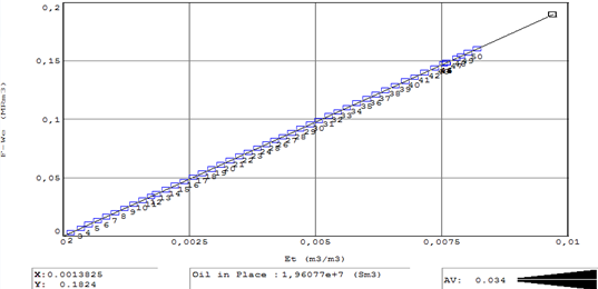
Figure5: Graphical plot result for estimating STOIP.
The STOIP value is shown in Figure 4. The results obtained from different graphs and tables are presented in Table 4.
| Methods used | Volumetric method (Sm3) | Material balance method (Sm3) |
|---|---|---|
| Initial Oil In Place (STOIP) | 67,639,727.94 | 19,607,700 |
| Recovery factor | 36,525,453.09 | 10,584,378 |
Table 4: Summary of the results obtained.
The volumetric method uses the petrophysical data which has supposed static. While the reservoir engineering material balances equation is a dynamic analytical tool for evaluating reserves volume through historical production.
Discussion
For this case study, it was question to make a comparison study between the volumetric method and the material balance method to choose the reliable method in the well F-12 of the Volve field (block 15/9). With the Volve field data available and the methodology used for this study, the following results obtained: The volumetric method gives estimated oil in place of about 67,639,727.94 Sand the reserve of 36,525,453.09 S. The STOIP estimated by using MBAL software is 19,607,700 Sand the reserve is estimated to 10,584,378 S. The volumetric method is used before there are sufficient production and/or pressure data to use the material balance method, so it does not integrate enough consistent data to estimate reserves as reliable as possible. The volumetric method may be subject to considerable uncertainty. Otherwise, material balance method utilizes reservoir engineering equations to calculate oil and/or gas initially in place and more. The reliability of these calculations depends on the accuracy with which the mathematical model and the available data simulate the reservoir under study. The major difference between these two methods is: The volumetric method is based on the assumption that the reservoir is static and the reservoir is homogeneous. This is the reason why volumetric method provides an overestimated reserve. The material balance method accounts for production and the resulting pressure decline. MBAL value for the oil originally in place is lower compared with its volumetric counter-part. This may signify the presence of a sealing fault (oil being trapped in undrained fault compartment or low permeability regions of the reservoir). So, the material balance method seems like the best method because of the amount and the type of production data used. It can be concluded that good evaluation of quantities in place is very difficult to make in the appraisal phase? Not necessarily, because a skillful analyst will use its data accurately. Yet it is necessary to be fully aware of the extent of the uncertainties in the field, and work with the concept of evaluate within reasonable limits.
Conclusion
In this paper, it was question to evaluate the best method for estimating reserves. This initiative comparison was concerned the chase of reliability in the estimation of reserves in well F-12 of Volve field. For that, estimation was first of all done by volumetric method by using petrophysical data. The second estimation was performed by material balance method by using PVT data, production history data and tank data carried inside MBAL software. It was found that the volumetric method gave estimated oil in place of about 67,639,727.94. So the reserve is equal to 36,525,453.09. While the stock tank original oil in place generated from MBAL software was 19,607,700 S, so the reserves is estimated to 10,584,378. From this comparative study, one can retain that material balance method is the best method and the accurate method because of the quality and quantity of data used. But volumetric method estimation is less reliable because it is applied early in the steps of field development. Volumetric method is based on the static nature of the reservoir and utilizing petrophysical and geological data determined under static conditions as the volume on a net pay basis. The net sand thickness as the formation sand thickness may not be considered as continuous. The material balance method assumes the reservoir as a tank and therefore does not take into account that it is static and homogeneous. However, even though the volumetric method is applied at the start of the development field, must be conclude that good evaluation of quantities in place is very difficult to make in the appraisal phase? Not necessarily because a skillful analyst will use his data accurately. Yet it is necessary to be fully aware of the extent of the uncertainties in the field, and work with the concept of evaluate within reasonable limits.
References
-
Desorcy GJ (1979) Estimation methods for proved recoverable reserves of oil and gas. 10th petoleum congress pp: 58.
-
Economides MJ, Boney C (2000) Reservoir Stimulation in Petroleum Production (éd. Reservoir Stimulation). Texas, Chinchester, USA: John Wiley & Sons LTD, pp: 1-30.
-
Guo B, Lyons WC, Ghalambor A (2007) Petroleum Production engineering A computer-Assisted Appraoch. Books ES, (Edn.).
-
John S (2018) Forecasting Oil and Gas Producing for Unconventional Wells 2nd (Edn.), Petro. Denver.
-
Boyun G, William C, Ali G (2007) Petroleum Production Engineering. 2nd (Edn.), Elsevier Science & Technology Books.
-
Bellarby J (2009) Well completion design, 1st (Edn.), Elsevier, Amsterdam, Nertherlands, pp: 304-367.
-
Groult J (1976) Notes for ENSPM lectures on geology, geophysics and production geology 23973: 24-25.
-
Leroy G (1979) Cours de geologie de production, ENSPM lectures, Ref 24(429) : 12-14.
-
Arli SM (2001) Estimation and classification of reserves of crude oil, natural gas, and condensate.Richardson: AIME.
-
Hsu CS, Robinson PR (2019) Petroleum Science and Technology, 1st(Edn.), Cham, Switzerland, Springer Nature AG.
-
Cook FJM, Graham M (2003) Hydrocarbon Exploration and production, 2nd(Edn.), Armsterdam, Nertherlands: Elsevier.
-
Szydlik T (1975) Prestack depth migration on the volve field, Stavanger: First break.
-
Rhys LA (1975) A proposed standard litho-stratigraphiy nomenclaturefor the southern sea. Norway, Applied science publishers.
-
Crumpton H (2018) Well control for completions and interventions. 1st (Edn.), Elsevier, Oxford.
-
John S (2018) Forecasting Oil and Gas Producing for Unconventional Wells 2nd (Edn.), Petro. Denver.
- Lessons to Learn: Trees are More than the Lungs of the World
- Community Forestry Enterprises as a Model for Sustainable Forest Development: The Case Of The "Baja Tarahumara" in Chihuahua, Mexico
- Ecological and Socio-Economic Impacts of Chromolaena odorata and Mesosphaerum suaveolens, Two Invasive Alien Species in Central and Southern Benin, West Africa
- Epigenetic Sustainability: Modeling the Human Factor as a Natural Resource through Science 4.0 and the NR3C1 Biological Pilot
- Growth-at-Risk: A Framework for Assessing Economic Vulnerability
- The Rural Territory as a Socioecological System for the Management of Public Policy for Sustainable Rural Development