Evaluation of Delbo Small Scale Irrigation Scheme Performance Southern, Ethiopia
Southern Nations, Nationalities and Peoples Region have launched a number of small-scale irrigation projects to help farmers achieve food self-sufficiency. However, because their systems' performances have not been assessed, it is unknown what level of performance they are capable of. Therefore, this study was conducted to determine the effectiveness of the Delbo small-scale irrigation system in southern Ethiopia. The result revealed that, the output per cultivated hectare was between 7668.96 and 31585.36 birr/ha, and the output per season's unit command area ranged between 5560 and 21583.33 birr/ha. The irrigation supply output per unit ranges between 1.0 and 3.32 birr/m3. The relative water supply (RWS) and irrigation water supply (RIS) were 2.03 and 2.75, respectively. This indicated that irrigation water was not in limited supply, and more water was diverted to the Delbo irrigation facilities. The average application efficiency of the chosen farmer's field was 53.3%, storage efficiency was 61.73%, distribution uniformity was 75.58%, and conveyance efficiency was 73.4%. Field I was more effective than Field II in terms of irrigation water management, while Field III was the least effective. One issue that must be addressed to ensure the sustainability of the schemes is to increase the management abilities of the users in order to improve the scheme's water use.
Introduction
In many nations, water scarcity is becoming a bigger issue. Being the primary consumer of water, the irrigation system is under pressure to release water for other uses and to develop ways to enhance performance [1]. A consistent and appropriate supply of irrigation water can boost agricultural output and ensure the economy’s health. The development of water for agriculture is a top priority in Ethiopia, but irrigation that is poorly planned and managed undermines attempts to improve lives and puts people and the environment at danger. According to recent estimates, Ethiopia has a total irrigable area of 625,819 acres [2]. The spread of small-scale irrigation was largely responsible for the rise in the irrigated area. However, Ethiopia’s current level of irrigation development pales in comparison to its potential. The challenge of comparing the performance of systems is not difficult given the numerous factors that affect how well irrigated agriculture performs, such as infrastructure design, management, climatic conditions, and socioeconomic contexts. Researchers have made significant progress in modernizing irrigation systems in response to the difficulties faced by irrigated agriculture, and these methods now include a variety of instruments for automation and equipment, strategies for field evaluation, and models for design and analysis [3]. Field assessments are crucial to enhancing the efficiency of surface irrigation because they offer the knowledge needed to enhance practices and systems. However, because they are so difficult to perform, they are rarely used [4]. Numerous field evaluations have been carried out by various scholars worldwide to address the issue of irrigation system performance, albeit to a lesser extent in Ethiopia [5]. In order to evaluate the effectiveness of the Delbo irrigation system in the southern region of Ethiopia, this study was carried out.
Methodology
General Descriptions of the Study Area
One of the 77 Woredas that can be found in Ethiopia’s
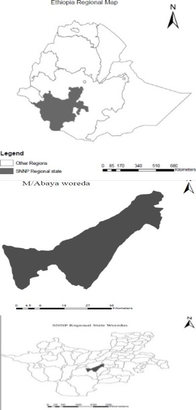
Southern Nations, Nationalities, and Peoples’ Region (SNNPR) is Mihrab Abaya. It is situated in the Gamo Gofa region and has a 1,613 km2 land area.
The woreda’s geographic center is M/Abaya, located 457 kilometers from Addis Abeba and 230 kilometers from Hawassa. The area is located at 1235 meters above sea level, 7.2 degrees north, and 38.0 degrees east, respectively. Lowland regions make up 62% of the woreda, followed by midland regions (27%), and highland regions (11%). The largest monthly mean rainfall is recorded from January to April, while the mean annual rainfall ranges from 543 mm to 887 mm. The woreda’s minimum temperature ranges from July to October at 19.5 degrees, while its maximum ranges from December to March at 33.2 degrees.
Description of the schemes
The Shefe River, which is the source of irrigation water, is a river that is fed by gravity from upper streams. The plan now consists of a 120 ha command area and 96 hectares of irrigated land. The Wajifo site and the Delbo site, two irrigation schemes with potential irrigable land areas of 425 ha and 300 ha, respectively, were discovered in the woreda. The town of M/Abaya lies close to Lake Abaya.
Crop Water Requirement (CWR) and Irrigation Requirement (IR)
The Woreda Agricultural Office provided information on the irrigated crops that were grown within the command area. Discussions with the farmers and the document obtained from the agriculture Office were used to determine the dates for planting these crops. Additionally, information on the average monthly rainfall was gathered from the Meteorological Agency’s Southern Zone. The CropWat model FAO [6] used input data such as climatic data, the area covered, and the planting date of each crop to calculate the CWR and IR for each irrigated crop for all cropping seasons. Using the CropWat computer program and estimated irrigation intervals for the primary crops cultivated in the system, the monthly net crop water requirement (CWR) and the net irrigation need (IR) were calculated for each irrigated crop. The Penman-Monteith approach was used in this application to determine reference evapotranspiration (ETo) on a monthly basis [7]. Using FAO recommendations, crop coefficients (Kc) were also created for the major crops [8]. Therefore, the crop water requirements at each growth stage were determined using the crop coefficients offered by the CropWat computer application.
Determination of soil physical properties
a. Soil textural characterization In order to represent the head, middle, and tail water consumers of the irrigation systems, three farmer fields were specifically selected. A total of 54 soil samples, 18 from each farmer’s field, were taken to assess the fields’ moisture levels. Before being placed in an oven that was kept at 105 oC, the soil samples were weighted and placed in an airtight container. The samples were dried in the oven for a whole day. Three rows of the field-one in the middle and two on either side-were used to obtain representative soil samples for each field. Undisturbed soil samples were taken from each field using soil core samplers. Before and after each watering session, the soil moisture statuses in each field were measured.
In order to apply this, soil samples were collected, dried in an oven at 105°C to constant weight, and then the bulk densities at the two depths were calculated. This was done right before irrigation and two days after irrigation, at depths of (0–30 cm and 30–60 cm, respectively).
b. Determination of Field capacity and permanent wilting points Both the field capacity (FC) and permanent wilting point (PWP) of each farmer’s field, as well as the soil texture of each farmer’s field, were determined in the laboratory using soil samples that were taken from the same depths as those described above.
c. Measurements of irrigation efficiency The amount of water diverted to each farmer’s fields, the amount of moisture stored and retained in the root zone of the crop, and how evenly the water is spread over the fields were all measured directly in the field during each irrigation event in order to evaluate how effectively the water was used by the chosen farmers. The following characteristics were computed using direct field measurements from soil samples that were also collected to be oven-dried for moisture assessment.
d. Conveyance efficiency
Flow rates in various field canal sections were measured to estimate conveyance efficiency. The associated discharges at the primary, secondary, and tertiary canals were measured using the Float (Velocity-Area) method. When using the floating method, 10 m long, somewhat uniform canal portions were selected, and floats were let go from the upstream point. Using a stopwatch, the floater’s average transit time throughout the 10 m canal length was calculated. The discharge rate was then estimated by multiplying the average cross-sectional area by the average velocity, which was computed as a ratio of canal length to average time. The conveyance efficiency was then computed as follows [9]: First, the total inflow into the conveyance system and the quantity of water provided by the conveyance system were determined.
*100 Total water supplied bytheconveyancesystem Conveyanceefficiency Ec totalinflowintotheconveyancesystem = ( ) e. Application efficiency The depth of water applied to each field (Da) was measured and considering the overall size of the field [10]. Two days after irrigation, the depth of water stored in the root zone (Ds) was determined as the difference between the after and before irrigation moisture contents of the soils. For this purpose, 18 soil samples (9 from the top and 9 from the subsoil layers) was taken at a depth of 0-30 cm and 30-60 cm water retained (stored) in the soil profile of the root zone, depth of soil (Ds), and the total depth applied to the field, Da, was determined by using the following equations [11].
( ) ( ) Average depth of water stored in the root zone Ds Ea *100 Average depth of water applied Da = f. Distribution efficiency For calculating the distribution uniformity, the effective root depth of the maize (i.e. up to 60 cm) was taken as the zone of distribution and three rows were selected along each field (one row from the center and two rows from opposite sides). Auguring was done at three points starting from the beginning to the end of the three rows at regular intervals. And at each selected point of the row, soil samples were collected from two depths (i.e. at 0-30 cm & 30-60 cm). Therefore, a total of 18 samples, 9 from the topsoil (i.e. 0-30 cm) and 9 from the sub-soil (_i.e._30-60 cm) were collected before and after each irrigation event. These procedures were repeated three times on each of the three farmers’ fields. After measuring the soil moisture contents of the soil samples gravimetrically, the depth of water stored in that particular soil layer Xi was calculated using the following equation.
* * 100 Wa WB X AS D − = After calculating the depth of water stored (as the difference between the after and before moisture content) at each point of the rows, the Distribution Uniformity (DU) can be determined. The DU is defined as the percentage of the average application amount received in the least watered quarter of the field. It is the ratio of the average depth infiltrated in the lower quarter of observations to the average depth of all observations [12].
X X DU = *100 Lq
m Where:
Lq X is the mean of the lower-quarter depth of water infiltrated (or caught) and m X is the mean depth of all water infiltrated (or caught) (i.e. the average of all the nine points of the entire field.
g. Water Storage Efficiency To evaluate how effectively the applied water could satisfy the water requirement (water storage capacity) of the crops and compensate the moisture depleted by ET can be evaluated using water storage efficiency (Es). Computation of the amount of water potentially required to fill the root zone to field capacity (Dreq) was determined using the equation 3.7 below and The Soil Testing Center result of FC was used to calculate the soil moisture deficit, SMD, before irrigation (Dreq). After knowing the values of Ds and Dreq, equations were employed to calculate the water storage efficiency (Es), which is sometimes referred to as water requirement efficiency (Er), [13].
Ds Es Dreq = ( ) 2
11 000 * * i Dreq SMD Wfci Wbi Asi Di = = = − ∑
Where: Ds = Amount of water added (stored in) to the root zone during the irrigation in (mm). Dreq = Amount of water potentially required to fill the root zone to field capacity (mm) SMD = Soil moisture deficit within RZ below field capacity before irrigation (mm) Wfci = Moisture content of the ith layer of the soil at field capacity (FC) on an oven-dry weight basis (fraction) Wbi =Moisture content of the ith layer of soil before irrigation on an oven-dry weight basis (fraction) Di = root depth (m) h. Evaluation of performance indicators Among many indicators of the minimum set for performance indicators, the following were used in this assessment: Relative Water Supply (RWS), Relative Irrigation supply (RIS), and output indicators. These are meant to characterize the individual system for water supply and finances [14]. These indicators can be mathematically described as follows:
Total water supply Relativewater supply Cropdemand =
irrigationsupply Relativeirrigationsupply irrigationdemand = i. Production performance indicators = / birr Production Output perunit command area ha Comand area =
3 birr Production Output perunitirrigationsupply m Diverted irrigationsupply =
3 birr Production Output per water consumed m Volumeof water consumed by ET To compute the total production of the scheme the crop types grown in the respective sites and their average yield per hectare which was obtained from farmers as well as the average market price of each crop yield per quintal was considered.
Results and Discussion
Soil physical properties
The physical characteristics of the soils of the study area are presented in Table 1 below.
The outcome in table 1 demonstrated that the bulk density was roughly the same throughout the entire field. Why, because a larger overall porosity was reported in the same textural class. A high volume of pore space is indicated by a low bulk density, whereas a low volume of pore space is indicated by a higher bulk density. It also demonstrated that the soil was clay loam in both the depth and the farm position or fields, with the exception of Field-2, which was situated at the middle farm and had a 0–30 cm of sandy clay loam (SCL) textural class. We can infer from this study that clay loam (CL) makes up the majority of the soil in the command area.
| Farmers field | Soil depth(cm) | Bulk density(gm/ cm3) | Particle size % | Textural class | FC %) | PWP( %) | PH | ||
|---|---|---|---|---|---|---|---|---|---|
| Clay | Silt | Sand | |||||||
| Field 1 | 0-30 | 0.98 | 33 | 38 | 29 | CL | 33 | 25 | 6.56 |
| 30-60 | 1.00 | 35 | 40 | 25 | CL | 32 | 23 | 6.08 | |
| Field 2 | 0-30 | 0.99 | 31 | 38 | 33 | SCL | 29 | 23 | 6.98 |
| 30-60 | 1.03 | 37 | 40 | 23 | CL | 32 | 25 | 6.33 | |
| Field3 | 0-30 | 1.02 | 32 | 36 | 32 | CL | 28 | 21 | 6.65 |
| 30-60 | 1.04 | 31 | 35 | 34 | CL | 27 | 22 | 6.55 |
Table 1: Soil physical properties of selected fields of Delbo irrigation project.
Note: CL=Clay Loam; SCL=Sandy Clay Loam Table 1: Soil physical properties of selected fields of Delbo irrigation project.
Soil moisture content
Before and after each watering session, the soil moisture statuses in each field were measured. To do this, measure the soil moisture to a depth of (i.e., 0-30 cm and 30-60 cm) immediately prior to irrigation and two days after irrigation. The only crop grown in the chosen fields was maize.
| Farmer’s field | Time of soil sampling | Soil moisture contents %volume | |
|---|---|---|---|
| Soil depth, cm | |||
| 0-30 | 30-60 | ||
| Field 1 | Before irrigation A fter irrigation | 29.8 30.4 | 32.3 35.3 |
| Field 2 | Before irrigation A fter irrigation | 30.1 33.2 | 33.2 34.4 |
| Field 3 | Before irrigation A fter irrigation | 28.2 29.1 | 29.8 30.3 |
Table 2: Average soil moisture contents before and two days after irrigation.
The available soil water holding capacity (ASW)
Crop yield suffers from too much or not enough soil moisture in the root zone. In actuality, when the soil moisture level surpasses the “field capacity” (the amount of soil water retained after the gravitational water has drained), the soil becomes waterlogged and the roots start to die from a lack of oxygen [15]. The plants, however, start to permanently wilt beyond the recovery point when soil moisture is at or below the “permanent wilting point” (the level at which the roots can no longer take water from the soil because the remaining water is being held too tightly by soil particles). The soil profile holds the water that plants may use, known as accessible soil water (ASW), between the field capacity and permanent wilting point.
Equation (3.14) below is used to calculate the field’s possible soil water storage capacity.
| Farmer’s field | ASW (cm) | ||
|---|---|---|---|
| Soil depth at 0-30cm | Soil depth at 30-60cm | ||
| Field 1 | 49.56mm | 22.56mm | 27.0mm |
| Field 2 | 39.45mm | 17.82mm | 21.63mm |
| Field 3 | 37.02mm | 21.42mm | 15.60mm |
Table 3: Crop type and yield for Delbo Irrigation Project 2009/10 year.
We can infer from the results that field Number 1 has more water accessible than the other fields because it is located near the head of the water supply.
Agricultural performance
Output per unit cropped area and unit of command area The results of output indicators measured based on the 2010 cropping calendar are presented in Table 3 below.
| Crop type (1) | Area ha) (2) | Yield (qt/ ha) (3) | Yield(qt) 4)=(2)*(3) | Price(birr/qt) (5) | Revenue(birr) (6)=(4)*(5) |
|---|---|---|---|---|---|
| Maize Potato Teff Onion Mango Pepper Banana | 40 | 70 | 2800 | 210 | 588000 |
| Cassava | 20 | 90 | 1800 | 120 | 216000 |
| 2 | 15 | 30 | 700 | 21000 | |
| 2 | 60 | 120 | 700 | 84000 | |
| 6 | 200 | 1200 | 200 | 240000 | |
| 2 | 20 | 40 | 3500 | 140000 | |
| 20 | 200 | 4000 | 200 | 800000 | |
| 4 | 150 | 600 | 200 | 120000 | |
| total | 96 | 593 | 9366 | 5330 | 2209000 |
Table 4: Crop type and yield for Delbo Irrigation Project 2009/10 year.
The output indication can be calculated using the following formula: Output per cropped area for the year 2009/10 = 2209000/96 = 23010.41 birr/ha. This assumes that the cropped area and command area during the cropping season 2017/18 were 96 ha and 120 ha, respectively. For the 2009/10 fiscal year, output per unit command area was 2209000/120, or 18408.33 birrs/ha. Other years’ output indicators were found to be comparable. The outcomes are shown in the figures 1 and 2 below.
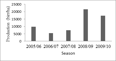
The findings revealed that the production per cropped hectare achieved ranged from 7668.96 to 31585.36 birrs/ ha. One may claim that compared to the other seasons, the income per cropped area in 2017–18 was higher. The farming intensities and the kinds of crops planted each year were thought to be the causes of this variance. While high-value cash crops covered a sizable amount of the irrigable region.
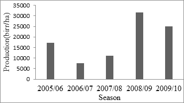
The outputs for each unit command area ranged from 5560 to 21583.33 birrs per hectare. These two seasons differed greatly from one another. The primary cause of this variance was noted to be the farmer’s increased production of high-value crops in 2008/2009. Additionally, there was a seasonal economic volatility that may have contributed to this increase in production.
a. Output per unit water consumed This indicator depicts the amount of output produced per unit of water used by the crop for evapotranspiration. In (birr/m3), the output per unit water supply during the season ranged from 0.72 to 2.97 birrs/m3. Low crop yield and bad agricultural practices may be to blame. The seasons differ significantly from one another. The difference in the area irrigated during the various seasons and crop choice could be the cause; the seasons with the highest value are those in which more vegetables are grown and there is a greater area irrigated.. The results are presented in Figure 4 below.
Low crop yields brought on by management practices and bad cropping patterns may be the cause of the season’s 2006/07’s low level of output. The outcome suggests that crop selection and cropping practices can affect productivity, which in turn lowers the crop’s gross profitability.
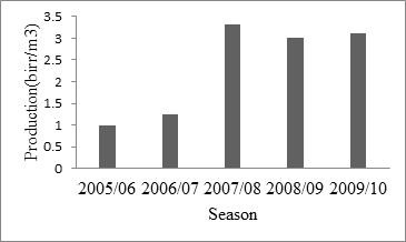
b. Output per unit irrigation water supply The output per unit irrigation water supply in birr/m3 for the year 2009/10 was calculated as; 2209000/603062.4 = 3.31 birr/m3. The results are given in Figure 5 below.
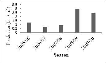
The findings show that the irrigation project’s output per unit irrigation water supply ranged from 1.0 birr/ ha to 3.32 birr/ha. In order to avoid overestimating or underestimating the crops’ pricing, average values were taken into consideration. Molden [14] recommendation of the same measure is likewise valid.
| Crop type | Area(ha) | Total rainfall, mm/ season | Effective rainfall, mm/season | Crop water requirement:S eason (mm/season) | Irrigation requirementm m/ season |
|---|---|---|---|---|---|
| Maize | 40 | 47.73 | 44.10 | 571.8 | 251.2 |
| Potato | 20 | 43.8 | 35.0 | 545.0 | 334.3 |
| Mango | 6 | 564.2 | 611.2 | 1507.7 | 701.8 |
| Banana | 20 | 884.0 | 709.2 | 1132.2 | 795.0 |
| Pepper | 2 | 444.6 | 355.9 | 502.8 | 265.5 |
| Teff | 2 | 468.9 | 375.9 | 475.6 | 178.8 |
| Onion | 2 | 232.9 | 186.7 | 270.5 | 98.3 |
| Cassava | 4 | 314.7 | 251.7 | 702.1 | 458.5 |
| total | 96 |
Table 5: CWR and IR of dominant crops at Delbo irrigation project 2009/10.
The weighted CWR per season and IR per season were calculated as the following equation CWR maize (area maize /area total)* CWR potato (area potato /area total)… IR maize (area maize /area total)*IR potato (area potato/ area total)… Where: CWRcrop: is the water requirement of a crop calculated and taken from the Table 4 Areacro_p_: is irrigated areas of the respective crops taken from the same Table 4 and Area total: is the total irrigated area (96 ha).
The weighted CWR result was 702.8 mm/season. To change the depth to the volume of CWR multiply it by the total irrigated area, i.e. 96 *104* 702.8* 10-3 = 6574688.0 m3 /season. The total irrigation requirement is calculated in the same way and the result is 315.69 mm/season i.e. 874688.0 m3 / season.
| Crop type | Area coverage(ha) | Percent of total area,% | Planting date | Irrigation intervals, days |
|---|---|---|---|---|
| Maize | 40 | 44.4 | May 07 | 7 |
| Banana | 20 | 22.2 | Jan 5 | 20 |
| Mango | 6 | 6.6 | Jan 9 | 15 |
| Potato | 20 | 22.2 | Jun 23 | 6 |
| Pepper | 4 | 4.4 | May 25 | 7 |
| Total | 90 | 100 |
Table 6: Area coverage planting date and irrigation interval of dominant crop.
The crop coefficients provided with the CropWat computer program are used (input: planting dates and growth length in days) to calculate the crop water requirement at each growth stage, and the computer program’s output was presented as shown in table 6 below. The net crop water requirement (CWR) and the net irrigation requirement (IR) were computed for each irrigated crop for the 2010 cropping season.
| Year | CWR (mm/ season) | Total rain (mm/ season) | Effective rainfall (mm/ season) | IR (mm/ season) | Area (m2) | CWR (m3/ season) | IR (m3/ season) | Depth of irrigationw ater diverted(mm) |
|---|---|---|---|---|---|---|---|---|
| 2005/06 | 324.52 | 184.6 | 165.8 | 264.67 | 790000 | 256370.8 | 2090890.3 | 323.98 |
| 2006/07 | 384.78 | 259.9 | 227.6 | 324.60 | 870000 | 334758.6 | 282402 | 654.09 |
| 2007/08 | 432.87 | 425.1 | 39.4 | 421.87 | 700000 | 303009 | 295309 | 765.89 |
| 2008/09 | 453.90 | 530.5 | 401.8 | 398.04 | 820000 | 372198 | 326392.8 | 876.09 |
| 2009/10 | 663.05 | 443.4 | 223.7 | 334.45 | 960000 | 636528 | 321072.0 | 789.32 |
Table 7: Seasonal CWR and IR.
c. Water delivery performance Using CropWat computer software, the water requirements of the main crops cultivated in the irrigation projects were calculated based on the farmers’ irrigation practices for each crop. The computation was done using the assumption that small-scale irrigation projects actually have an irrigation efficiency of 45% [16]. When additional research is done, this number can serve as a standard. The performance of water distribution was assessed using two indicators: relative water supply (RWS) and relative irrigation supply (RIS). Table 6 below lists the net crop water requirement as well as the irrigation requirement.
d. Relative water supply (RWS) An average relative water supply (RWS) value was found to be 2.36 for the period of 2005/06 up to 2009/10. As shown below, the RWS values of the whole season were higher than what can be considered an ideal value, i.e., 1.0. In the year 2005/06, water diverted to the irrigation scheme was slightly lower than the other season of crop water demand. Conversely, values less than 1.0 suggest that crops are not receiving adequate irrigation water, while values more than 1.0 suggest that there is enough water available overall to meet crop demand [17]. The average RWS value for the years 2005–06 through 2009–10 was determined to be 2.36. The RWS values for the entire season were higher than 1.0, which is regarded as an ideal value, as can be seen below. The amount of water diverted to the irrigation scheme in 2005–06 was marginally less than the crop water demand in preceding seasons. This suggests that there is insufficient watering of the crops.
Cakmak [18] report that for five irrigation schemes in the State Hydraulic Works 10th Region of Turkey over the 1997–2001 period, the relative water supply (RWS) values ranged from an average of 1.65 to 4.51. In terms of relative water supply (RWS), the Malaysia-Sg. Manik (4.9) and Malaysia-Mada (0.37) irrigation systems had the highest and lowest values. The results of RWS are presented in Figure 6.
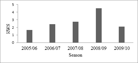
Figure 6 illustrates how the strategy has provided too much water during the seasons under consideration. This suggests that the cropping pattern selected in the various years’ supply is sufficient to satisfy demand. Of course, in order to determine the net supply gained, water losses must be taken into consideration; otherwise, the result may be less than this.
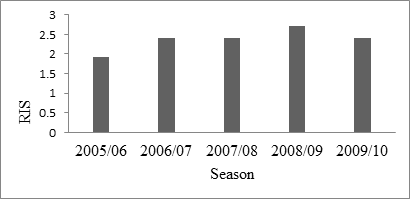
e. Relative irrigation supply (RIS) An indicator of the whole irrigation scheme’s efficiency is the RIS. Due to the fact that it contrasts the irrigation water required with the water supplied. The statistics in Table 6 above were used to compute the relative irrigation water supply. Figure 7 below displays the RIS results.
value greater than one indicates that too much water is being supplied, waterlogging may result, which would have a detrimental effect on yields. A score less than one indicate that less irrigation water was provided than was necessary. A number of 1.0 or above signifies that the irrigation supply met or exceeded the necessary standards. The findings show that farmers have applied more than enough irrigation water to meet crop demand during the whole season. Moreover, the 2005–06 year had the lowest recorded value of RIS, 1.92. There was most likely less rainfall, less maintenance done to the canal system, less organizational weakness, a different kind of crop being farmed, and so on throughout that time.
Irrigation efficiency indicators
a. Application efficiency Application efficiency is computed as the ratio of moisture added to the soil profile due to irrigation to the total water supplied to the farm or the ratio of moisture retained due to irrigation with total water added to the field.
- A plentiful supply of water was indicated by the higher relative irrigation supply (RIS) values. A RIS value of greater than 1.0 shows that the irrigation supply by the canal is sufficient to meet the crop demand; a value closer to one is preferable than one that is higher or lower [14]. Since a
- Farm position
- Farm size(ha)
- Time of irrigation(hr)
- Flow rate(l/s)
- Field 1
- 0.8
- 8
- 7.5
- 204
- 58.09
- 30.2
- 52.4
- Field 2
- 0.5
- 8
- 7.8
- 224
- 44.82
- 28.91
- 64.5
- Field 3
- 0.25
- 8
- 6.8
- 195
- 78
- 33.68
- 43
- Average 53.3%
Table 8: Calculated application efficiency.
The outcome demonstrated that, in accordance with the US soil conservation service range of 55% to 70%, field-3 falls short of the achievable application efficiency for surface irrigation systems. Numerous studies believe that the scheme’s average water application efficiency (Ea), of 53.3%, is insufficient and hence inefficient. The result obtained is consistent with the findings of Solomon (1988), FAO [19], the command area’s water application efficiency is deemed inadequate due to its value being less than 60%. The three farmer’s fields that were chosen have substantially lower application efficiency than the Tekeze basin’s community- based irrigation findings, which are 65% and 85% [20]. Wahaj [21] states that for furrow irrigation, the water application efficiency values should be 65–85%. These are seasonal values that should be achievable with appropriate design and management practices. In contrast, Solomon [22] recommended that the achievable application efficiency for furrow irrigation fall between 60 and 75 percent. Thus, the scheme’s water applications were deemed inappropriate; this suggests that farmers overwatered their crops, leading to increased deep percolation and runoff losses. High deep percolation losses are the main reason for the reduced water application efficiency, according to measurements and observations made in the field. The field observations of the farmers’ shallow water wells, which are dispersed over the whole command area, provide evidence for this.
b. Conveyance efficiency Water was transported from the river’s source to fields or farms for crop usage via a network of canals, watercourses, and channels. The system’s water conveyance efficiency was assessed using conveyance efficiency. It was also used to gauge how well the conduits carrying water to the field were working.
| Field measurement | Station-1 discharge | Flow measurement | Station-2 discharge(m3/s) | Distance between the stations(m) | Conveyance efficiency (%) |
|---|---|---|---|---|---|
| point | (m3/s) | point | |||
| Main canal | |||||
| 1-M | 0.621 | 2-M | 0.502 | 380 | 80.83 |
| 2-M | 0.567 | 3-M | 0.503 | 420 | 88.71 |
| 3-M | 0.492 | 4-M | 0.321 | 400 | 65.24 |
| 4-M | 0.521 | 5-M | 0.432 | 420 | 82.91 |
| Secondary canal | |||||
| 1-S | 0.23 | 2-S | 0.193 | 450 | 83.91 |
| 2-S | 0.156 | 3-S | 0.103 | 430 | 66.02 |
| 3-S | 0.143 | 4-S | 0.102 | 400 | 71.32 |
| 4-S | 0.102 | 5-S | 0.074 | 420 | 72.54 |
| Tertiary canal | |||||
| 1-T | 0.155 | 2-T | 0.118 | 400 | 76.12 |
| 2-T | 0.109 | 3-T | 0.077 | 420 | 70.64 |
| 3-T | 0.109 | 4-T | 0.089 | 380 | 81.65 |
| 4-T | 0.119 | 5-T | 0.088 | 400 | 73.94 |
| 5-T | 0.128 | 6-T | 0.087 | 420 | 67.96 |
| 6-T | 0.124 | 7-T | 0.098 | 380 | 79.03 |
| 7-T | 0.121 | 8-T | 0.086 | 400 | 71.07 |
| 8-T | 0.123 | 9-T | 0.076 | 420 | 61.78 |
| 9-T | 0.098 | 10-T | 0.071 | 440 | 77.55 |
| 10-T | 0.087 | 11-T | 0.064 | 380 | 73.56 |
| 11-T | 0.076 | 12-T | 0.055 | 420 | 72.36 |
| 12-T | 0.076 | 13-T | 0.054 | 400 | 71.05 |
| 13-T | 0.076 | 14-T | 0.054 | 440 | 71.05 |
| 14-T | 0.072 | 15-T | 0.05 | 440 | 69.44 |
| 14-T | 0.072 | 15-T | 0.05 | 440 | 69.44 |
| Average | 73.41% |
Table 9: Calculated conveyance efficiency.
The outcome demonstrated that the scheme’s average conveyance efficiency was 73.41%. Nevertheless, considering that high channel efficiency for the field was discovered. The plan conveyance efficiency is in line with research findings from the Food and Agriculture Organization (FAO) [23] conducted in Egypt in 2002, which projected that water losses via canals accounted for 25-50% of all water losses. Since the scheme’s average application efficiency was 73.41%, conveyance losses indicate that, of the total water harvested and stored, the remaining portion that is, 26.59% is lost. This does have implications for locations where water scarcity exists.
c. Distribution uniformity Water distribution uniformity measures the extent to which water is uniformly distributed and stored in the effective root zone soil along the irrigation run. The distribution uniformity indicates the magnitude of the distribution problem.
| Irrigation | |||||||||||
|---|---|---|---|---|---|---|---|---|---|---|---|
| Farm position | event | Depth of water stored at each sampling point up to the effective RZ, X (mm) | |||||||||
| X1 | X2 | X3 | X4 | X5 | X6 | X7 | X8 | X9 | - | ||
| X m | |||||||||||
| Field-1 | 1st | 28.18 | 25.01 | 28.38 | 32.74 | 27.49 | 36.57 | 22.32 | 38.83 | 29.09 | |
| 2nd | 32.25 | 27.03 | 23.61 | 31.38 | 26.89 | 35.5 | 33.09 | 34.13 | 27.46 | ||
| 3rd | 27.47 | 26.29 | 26.83 | 33.82 | 26.42 | 32.41 | 30.38 | 28.18 | 30.01 | ||
| 29.3 | 26.7 | 24.74 | 33.72 | 25.8 | 30.86 | 29.49 | 31.71 | 28.51 | |||
| DU of Field-1 (%) | |||||||||||
| Field-2 | 1st 2nd 3rd | 28.17 | 27.95 | 25.81 | 26.47 | 32 | 24.51 | 24.17 | 33.27 | 28.87 | |
| 30.37 | 28.35 | 28.1 | 25.53 | 30.42 | 20.21 | 31.64 | 28.2 | 21.97 | |||
| 31.04 | 18.05 | 29.7 | 28.53 | 35.71 | 20.23 | 17.3 | 29.59 | 28.64 | |||
| 29.86 | 24.78 | 27.87 | 26.84 | 32.72 | 21.93 | 24.87 | 30.33 | 26.49 | |||
| DU of Field-2(%) | 1st 2nd 3rd | 36.58 | 35.56 | 34.93 | 25.94 | 36.79 | 34.82 | 34.48 | 36.06 | ||
| Field-3 | 1st 2nd 3rd 35.78 | 34.98 | 28.67 | 33.56 | 20.39 | 29.19 | 32.11 | 33.33 | 34.4 | 30.57 | |
| 35.73 | 30.23 | 30.18 | 27.92 | 28.82 | 35.04 | 36.12 | 29.09 | 34.05 | |||
| 31.35 | 32.2 | 24.75 | 33.7 | 33.25 | 34.87 | 32.51 | 32.02 | 30.04 | |||
| DU of Field-3 (%) |
Table 10: Depth of water stored (caught) within the effective RZ of each farm.
The irrigation schemes’ average distribution uniformity was 75.58%. The distribution homogeneity exceeds the 70% value discovered in the irrigation systems of the Western United States by Pitts [24]. FAO [6] proposed that distribution uniformity (DU) of 65% was considered “sufficient” while a DU of 30% was considered “poor” when it came to average rotational supply with management and communication. However, SJVDIP [25] estimates that the furrow irrigation distribution uniformity should be between 80 and 90 percent, meaning that the distribution uniformity is inefficient.
d. Storage efficiency The water storage efficiency refers to how completely the water needed before irrigation has been stored in the root zone during irrigation.
| Field position | Depth of irrigation water required(mm) | Depth of irrigation water retain in 60cm soil | Storage efficiency (%) |
|---|---|---|---|
| Dreq | depth(mm) | ||
| Field-1 Field-2 | 48.9 | 34.8 | 71.1 |
| Field-3 | 72.1 | 52.6 | 72.9 |
| 33.4 | 17 | 50.8 | |
| Average | 64.90% |
Table 11: Calculated storage efficiency (%).
The irrigation schemes’ average storage efficiency was 64.9%. Lesley [26] states that the irrigation scheme’s overall water storage efficiency, or 96.63%, is taken to be the maximum figure that can be attained for furrow irrigation. According to Michael [9], the potential values for furrow irrigation range from 85% to 100%. Storage efficiency values are the highest values that can be achieved globally. This indicates that the goal of irrigation water storage-refilling the root zone to field capacity-is, in some way, perceived as having been accomplished.
Conclusions
The purpose of the study was to evaluate the effectiveness of small-scale irrigation projects in Ethiopia’s south. Various metrics have been employed to assess the system’s performance in comparison to other systems operating in comparable environments or accomplishing its primary goals. The 2007–08 season outperformed the previous one in terms of output per unit of command area and output per unit of cropped area. This was attributed to both favorable market conditions and effective management practices. More water was redirected to the Delbo irrigation schemes, according to the average relative water supply (RWS) and relative irrigation supply (RIS), which showed that irrigation water is not a scheme restriction. i.e., when the amount of water available exceeded the amount required in every field, it was clear that the irrigation water was not applied consistently and effectively. The total production of all crops was not combined into an internationally tradable single crop; consequently, the agricultural performance indicator is not compared with other countries worldwide. Levine [27] stated that water supplied more than 2.5 times the net requirement was an indication of inappropriate water management. The 2008/09 cropping season’s diversified cropping pattern led to the relatively higher value of output per unit of cultivated land and command area, while the lower value in the other year was primarily caused by crop choice and management issues [28, 29, 30, 31]. According to the study, farmers simultaneously produce comparable crops, which causes a market exchange among them. Therefore, marketing and other essential facilities like price, information, storage, marketplace, production diversity, and consumer preference should be taken into account in any future interventions to promote crop production, especially cash crops [32, 33, 34, 35, 36]. Farmers are applying excess water to their fields, and the findings of the water delivery indicators indicated that there is no water shortage for the plan. To enhance effective water use and production, water management must be improved [37, 38]. Regarding the farmers’ efficiency in applying water, the irrigation plan is deemed inadequate [39, 40, 41, 42]. As a result, a significant amount of water is lost from the canals both temporarily and steadily. According to the results of water storage efficiency, irrigation water replaced roughly 65% of the moisture that evapotranspiration had reduced below field capacity (FC). According to the irrigation scheme’s performance indicators, the season of 2008/09, when farmers were cultivating more high-value crops, performed well in terms of production per unit of land and water, respectively. However, the other season’s performance didn’t show an increasing or decreasing trend due to poor cropping practices and low input utilization [43, 44, 45]. These data were gathered between 2005/06 and 2009/10. Inefficient water consumption was shown by the water use performance indicators, indicating that more effort has to be done to increase water use efficiency [46].
Recommendation
The outcomes have led to the following suggestions being made to enhance the performance of the irrigation scheme:
- The irrigation projects have a significant conveyance loss. To lessen the seepage loss, it is therefore strongly advised to line or build canals using concrete or masonry.
- Upon examining the farmers’ fields, it was discovered that although application efficiencies were low, distribution efficiencies were strong. Therefore, it is necessary to apply correct irrigation schedule in order to improve the effectiveness of the irrigation systems.
- Emphasis should be placed on crop selection, irrigation water management, and input utilization. Establishing strategically located market access improves the scheme’s performance. References
1. Malano HM, Burton I, Makin (2004) Benchmarking performance in the irrigation and drainage sector: a tool for change. Irrigation and Drainage 53(2): 119-133.
2. Fitsum Hagos, Godswill M, Namara RE, Awulachew SB (2009) Importance of Irrigated Agriculture to the Ethiopian Economy: Capturing the Direct Net Benefits of Irrigation. IWMI Research Report 128.
3. Pereira LS (1999) Higher performance through combined improvements in irrigation methods and scheduling: a discussion. Agricultural Water Management 40(2): 153- 169.
4. Pereira LS (2005) Water and agriculture: Facing water scarcity and environmental Challenges. Agricultural Engineering International: the CIGR Journal of Scientific Research and Development.
5. Melaku Mekonnen (2005) Performance evaluation of Bato Degage surface irrigation systems, East Shewa
Zone. An MSc thesis, Alemaya University.
6. Food and Agriculture Organization (FAO) (1992) Ninth meeting of the East and Southern African Sub-committee for soil correlation and land evaluation. Soil Bulletin No.70. Rome, Italy.
7. Allen RG, Pereira LS, Raes D, Smith M (1998) Crop Evapotranspiration: - Guidelines for Computing Crop Water Requirements. Irrigation and Drainage Paper, pp: 56.
8. Doorenbos J, Kassam (1986) Guidelines for predicting crop water requirements, Irrigation and Drainage Paper 24, Food and Agriculture Organization of the United Nations, Rome, pp: 179.
9. Michael AM (1997) Irrigation Theory and Practice. Evaluating Land for Irrigation Commands. Vikas Publishing House Pvt. Ltd, New Delhi, India.
10. Mishra RD, Ahmed M (1990) Manual on Irrigation Agronomy. Oxford and IBH Publishing Co. Pvt. Ltd. New Delhi, Bombay, Calcutta, India.
11. James LG (1988) Principles of Farm Irrigation System Design. John Wiley and Sons, New York.
12. Walker WR 2003) SIRMOD III: Surface irrigation simulation, evaluation, and design.
13. Jurriens M, Lenselink MK (2001) Straightforward furrow irrigation can be 70% efficient. Irrigation and Drainage paper 50(3): 195-204.
14. Molden DJ, Sakthivadivel R, Perry CJ, Fraiture C de, Kloezen WH (1998) Indicators for comparing the performance of irrigated agricultural systems. Colombo, Sri Lanka: International Water Management Institute, pp: 1-26.
15. Ley TW, Stevens RG, Topielec RR, Neibling WH (1994) Soil Water Monitoring and Measurement. Paper PNW0475. Pacific Northwest Cooperative Extension Publication.
16. Chancellor FM, Hide JM (1997) Small Holder Irrigation: Ways Forward.Guidelines for Achieving Appropriate Scheme Design.
17. Beyribey M (1997) Devlet sulama ebekelerinde system performance the erlendirilmesi. A.Ü. Ziraat Fakültesi Yayınları No: 1480, Bilimsel Ara_tırma ve _ncelemeler: 813, Ankara, Turkey (in Turkish).
18. Çakmak B, Beyribey M, Yıldırım YE, Kodal S (2004) Benchmarking performance of irrigation schemes: A case study from Turkey. Irrigation and Drainage 53(2):
155-163.
19. Food and Agriculture Organization FAO (1989) Guidelines for Designing and Evaluating Surface Irrigation Systems. Irrigation and drainage paper, pp: 45.
20. Mintesinot B, Mohammed A, Atinkut M, Mustefa Y (2005) Community- Based Irrigation Management in the Tekeze Basin: Performance Evaluation. A case study on three small-scale irrigation schemes (micro dams, A collaborative project between Mekelle University, ILRI & EARO.
21. Wahaj R (2001) Farmers actions and improvements in irrigation performance below the mogha: How farmers manage water scarcity and abundance in large scale irrigation systems in South-Eastern Punjab, Pakistan. Ph.D. dissertation. Wageningen University,
22. Solomon KH (1988) Irrigation Systems and Water Application Efficiencies. WATERIGHT. Center for Irrigation Technology. California State University, Fresno, California.
23. Food and Agriculture Organization (FAO) (2002) Agricultural drainage water management in arid and semi-arid areas. FAO Irrigation and Drainage Paper, pp: 190.
24. Pitts DK, Peterson G, Gilbert, Fastenau (1996) Field assessment of irrigation system performance. American Society of Agricultural Engineers 12(3): 307-313.
25. SJVDIP (San Joaquin Valley Drainage Implementation Program) (1999) Source reduction technical committee report. Department of Water Resources. Sacramento, United States of America.
26. Lesley W (2002) Irrigation Efficiency_._ Irrigation Efficiency Enhancement Report No 4452/16a, March 2002 Prepared for Land WISE Hawke’s Bay. Lincoln Environment. The USA.
27. Levine G (1982) Relative Water Supply: An Explanatory Variable for Irrigation System. Technical Report No: 6, Cornell University, Ithaca, New York, USA.
28. Bos, MG, Burton MA, Molden DJ (2005) Irrigation and drainage performance assessment: Practical guidelines. CABI Publishing, U.K.
29. Bos, Marinus G (1997) Performance Indicators for Irrigation and Drainage. In Irrigation and Drainage Systems. Kluwer Academic Publishers 11: 119-137
30. Bright J, Carran P, McIndoe I (2005) Designing effective and efficient irrigation systems. Report No 2788/1, prepared for MAF Policy. Lincoln Environmental, a division of Lincoln Ventures Ltd.
31. Burton M, Molden D, Skutsch J (2000) Benchmarking irrigation and drainage system performance, Position paper, IPTRID- FAO-WORLD BANK, Working Group on Performance Indicators and Benchmarking, Report on a Workshop, 3-4 August 2000, FAO, Rome, Italy.
32. Clarke D (1998) CropWat for Windows: User Guide. Version 4.2. University of Southampton, UK.
33. Clemmens AJ (2006) Improving irrigated agriculture performance through an understanding of the water delivery 1993 process. Irrigation and Drainage 55: 223-234.
34. David J, Molden R, Sakthivadivel, Christopher JP, Charlotte de Fraiture, et al. (1998) Indicators for Comparing Performance of Irrigated Agricultural Systems. International Water Management Institute, pp: 26.
35. Douglas LV, Juan AS (2001) Transfer of Irrigation Management Services. Guideline: Irrigation and Drainage Paper, pp: 58.
36. Food and Agriculture Organization (FAO) (1997) Small-Scale Irrigation for Arid Zones: Principles and Options.
37. Gillot PW, Bird JD (1992) Review of performance indicators for irrigation management: adequacy and equity. Hydraulic Research, Wallingford, England, report OD/TN.
38. Hasan D, Hakan B, Hayrettin K (2003) Assessment of Irrigation Schemes with Comparative Indicators in the Southeastern Anatolia Project. Turkish Journal of Agriculture and Forestry 27(5): 293-303.
39. Karaa FK, Tarabey N (2005) attempt to determine some performance indicators in the qasmieh ras – el- ain irrigation scheme (Lebanon), Lake Share Communities Union, Association of Irrigation Water Users in South Bekaa Valley, Lala, Lebanon.
40. Kloezen WH, Garces-Restrepo C (1998) Assessing Irrigation Performance with Comparative Indicators: The Case of the Alto Rio Lerma Irrigation District, Mexico.
41. Koshi Y, Hajime T, Hiroaki S, Osamu T, Katsuhiro H (2002) Evaluation of irrigation efficiency at km6 project site, Laos, national institute for rural engineering Japan.
42. Lemma Dinku (2004) thesis on Smallholders’ Irrigation Practices and Issues of Community Management: The Case of Two Irrigation Systems in Eastern Oromia, Ethiopia.
43. Merriam JL, Nugteren J, Keller J (1983) Farm irrigation system evaluation: A guide to management”, Utah State University, Logan, Utah.
44. Pereira LS, Trout TJ (1999) Irrigation Methods, Land and water engineering, CIGR handbook of agricultural engineering.
45. Stijn S, Marijke D, Haese B, Jeroen B, Luc D’Haesea (2007) Technical efficiency of water use and its determinants, study at small scale irrigation schemes in North- West Province, South Africa Montpellier, France.
46. Yusuf Kedir (2003) Assessment of small scale irrigation using comparative performance indicators on two selected schemes in upper Awash River valley thesis, Haramaya University.
- Lessons to Learn: Trees are More than the Lungs of the World
- Community Forestry Enterprises as a Model for Sustainable Forest Development: The Case Of The "Baja Tarahumara" in Chihuahua, Mexico
- Ecological and Socio-Economic Impacts of Chromolaena odorata and Mesosphaerum suaveolens, Two Invasive Alien Species in Central and Southern Benin, West Africa
- Epigenetic Sustainability: Modeling the Human Factor as a Natural Resource through Science 4.0 and the NR3C1 Biological Pilot
- Growth-at-Risk: A Framework for Assessing Economic Vulnerability
- The Rural Territory as a Socioecological System for the Management of Public Policy for Sustainable Rural Development