Daily Water Surplus Variability between the Mediterranean, Semi-Arid and Arid Climates
Water surplus in a water balance is the fraction of precipitation which does not evaporate and not stored in the soil and includes both surface runoff and deep percolation. The annual course of the distribution of days with water surplus was estimated by a simple water balance model, which combines daily rainfall data, pan evaporation and soil water properties. The model was run using available published daily rainfall series and pan evaporation from ten Israel Meteorological Service stations, representing various climatic regions of Israel and using 21 different soil depths to simulate different root zone depths. The calculated daily water surplus series enable to evaluate the probability and amount of water surplus on each day of the year. The model output can be used in various hydrological models and be applied to other regions with similar conditions, without any special adjustment and may serve as an important tool for planners. This information is crucial for evaluation of the timing of occurrence of geomorphological and hydrological processes which depend on water surplus in various seasons. The annual aggregation of the water balance components provides a general view of the hydrological conditions of the different stations. The probabilistic representation of the results enables a comparison among stations with different rainfall regimes and soil types.
Introduction
The climate, soil and vegetation systems are coupled via complex of physical, chemical, and biological processes. The spatial and temporal heterogeneity of these biophysical factors, and their interactions, make the hydrological processes of each region unique.
The fundamental equation in hydrology is likely to be the water balance equation which is an arithmetic expression of the relationship between the various components of the hydrologic cycle [1, 2, 3]. The difference between total input and output will be balanced by the change in soil water storage. Therefore, this change in soil water storage is the result of the precipitation minus evaporation minus water surplus. Hence, surplus is the fraction of precipitation which does not evaporate and is not stored in the soil storage and includes both surface runoff and deep percolation.
In a classical empirical study Budyko [4] provided a simple framework for describing the control of climatic forcing on hydroclimatic regime, showing an asymptotic behavior in observed water balances as one progresses from energy limited to water limited systems. Eagleson [5], in his more comprehensive analysis of hydroclimatology, addressed a number of additional controls on evaporation and runoff, including storm and interstorm properties and soil and vegetation properties. Milly [6] have used an idealized model of water balance to explore the basis of regional variability of water balance, explaining the role of intraseasonal soil water storage.
The present work is motivated by the desire to explore water balance variability at daily timescale, in the context of the controlling climate and soil characteristics dissimilarities in different climatic regions.
Water balance models can have different levels of complexity, depending on the aims and methodology of the study and data availability. In the simplest case, the only input data required are rainfall, potential evapotranspiration and soil-water holding properties. There are a number of variations to the simple model depending on conceptualization of the system and methods for estimating evapotranspiration [7, 8, 9, 10, 11, 12]. It is important to notice that increasing model complexity does not necessarily improve accuracy [13, 11].
In the present study, we used a simple water balance model, which has been used, tested and verified in many studies. We adopted this model using available published daily rainfall series and daily pan evaporation measurements to estimate the remaining water balance parameter of daily surplus water (SW) in various climatic regions. In order to have a general view of the hydrological conditions of the different stations and in order to compare the results to other regions the daily water balance parameters were, also, aggregated to annual data.
Data and Methods
Study Area
Israel is located at the easternmost part of the Mediterranean Sea. About 66% of the rainfall is in winter (DJF). The remaining falls in autumn (SON) and spring (MAM), while the summer (JJA) is dry. Therefore, the hydrological year is used, i.e. the 1 September of each year is considered as the first day of the year and 31 August of the following year is considered as the 365th day. In the few cases in which it rained on 29 February the amount was assigned to 28 February.
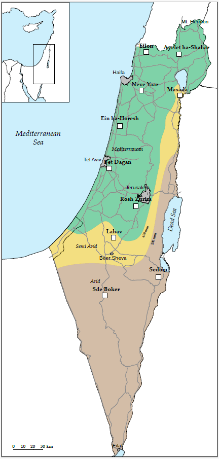
Rainfall variability is very large both at the spatial and temporal scales. Annual totals vary from more than 1300 mm on Mt. Hermon in the north to less than 25 mm at Eilat in the south (Figure 1). At the temporal scale, there is a very large variability regarding the timing of the rainfall within the rainy season with a range of over two months in the mid- season date (e.g. Reiser and Kutiel [14, 15]).
Data
Ten stations out of the Israel Meteorological Service (IMS) network were selected to represent the various climatic conditions in Israel. All selected stations have daily rainfall and daily pan evaporation series over a period of at least 22 years (Figure 1, Table 1). The IMS defines a rainy day as a 24 hrs. period, starting at 08:00 LT (06:00 UTC) and ending at 07:59 LT of the following day, with a measurable rainfall amount of at least 0.1 mm. Daily pan evaporation [mm] was measured by the changes of the water height in a Class A pan.
| Climatic region | Altitude a.s.l | Data series length | Mean annual rainfall* | Mean annual rain days* | Mean annual pan evaporation* | Soil type** | |
|---|---|---|---|---|---|---|---|
| (m) | (years) | (mm) | (mm) | ||||
| Eilon | Mediterranean | 300 | 41 (1979-2019) | 811.0 | 74 | 1674.4 | Terra Rossa (Rhodoxeralfs) |
| Ayelet ha-Shahar | Mediterranean | 170 | 44 (1970-2013) | 462.7 | 63 | 1953.6 | Alluvial Soil (Vertic Xerofluvents) |
| Neve Yaar | Mediterranean | 115 | 22 (1994-2015) | 549.7 | 59 | 1663.3 | Brown Alluvial Soil (Chromoxererts) |
| Masada | Semi-Arid | -200 | 36 (1975-2010) | 374.7 | 55 | 1732.7 | Rendzina Soil of Valleys (Calciorthids) |
| Ein ha-Horesh | Mediterranean | 15 | 44 (1976-2019) | 569.6 | 61 | 1675.8 | Brown Red Sandy Soil (Haploxeralfs) |
| Bet Dagan | Mediterranean | 31 | 56 (1964-2019) | 545.8 | 58 | 1735.3 | Alluvial Soil (Vertic Xerofluvents) |
| Rosh Zurim | Mediterranean | 950 | 48 (1971-2018) | 541.8 | 56 | 1835.4 | Terra Rossa (Rhodoxeralfs) |
| Lahav | Semi-Arid | 460 | 42 (1978-2019) | 304.2 | 45 | 1833.4 | Mediterranean Brown Forest (Haploxerolls) |
| Sedom | Arid | -388 | 48 (1964-2011) | 40.6 | 15 | 3839.0 | Desert Alluvial Soil (Torrifluvents and Salorthids) |
| Sde Boker | Arid | 475 | 53 (1967-2019) | 92.9 | 28 | 2365.9 | Loess Raw Soil (Xerollic Camborthids) |
Table 1: Characteristics of the rainfall stations.
The Water Surplus Model
Water surplus in the water balance model described in Equation [1] is the fraction of rainfall that exceeds potential evaporation and is not stored in soil. The simple model used in this study does not distinguish between surface runoff and deep percolation and includes both. All calculations below were done on a daily basis using daily data. WSj = Rj – PEj – (SMj – SMj-1) [1]
Where WS is water surplus [mm], R is rainfall [mm], PE is potential evaporation [mm], SM is soil moisture [mm] for a given depth and j denotes the number of the day in the hydrological year (1=1 Sep., 2=2 Sep.… 365=31 Aug.).
Soil moisture is treated in a water balance as a storage term; therefore it should be related to depth, usually root zone depth. In that zone, besides direct evaporation, the plant roots can extract water and remove it by evapotranspiration. Below root zone the water movement is dominated by gravity and may reach the watertable and then discharges into streams, recharge the groundwater or both. Soil depth may vary due to different factors such as slope, land use, parent material, weathering rate, climate, vegetation cover, upslope contributing area, and lithology [16, 17, 18]. As a result, root zone depth has highly spatial variability including cases where the soil is shallower than the usual depth of root penetration. Soil depth in the Mediterranean region frequently vary significantly over small distance and a microenvironmental mosaic is common in the ecosystems of that region, where geological formations, topographical conditions and changes in types of bedrock are very frequent [19, 20] and hence, in order to represent a wide range of possibilities, 21 soil depths were selected: 10 mm and from 25 mm to 500 mm with increments of 25 mm.
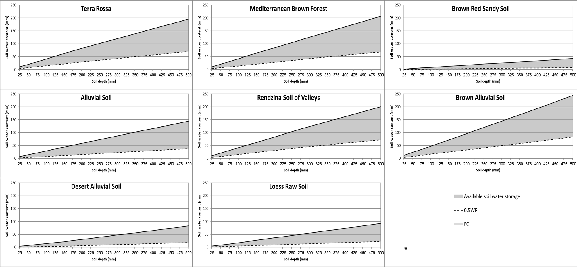
The ability of the soil to contain water is influenced by the soil properties, such as texture, structure, type of clay and organic matter content [21]. Several terms are used to define the water storage capacities of soils under different conditions. “Saturation” is the highest water content that the soil can hold, the matric potential is 0 bars and all the soil pores are filled with water. But, this is a temporary state which exists once in a while during a heavy rainstorm. Actually, upper limit is when the large soil pores drained out under the influence of gravity and the drainage becomes negligible. The amount of water remaining is called Field Capacity - FC. It roughly corresponds to a matric potential of -0.33 bars (-33 kPa). Wilting Point – WP is the soil water content that is held so tightly by the soil matrix that roots cannot extract sufficient moisture and a plant will wilt. For many cultivated plants the water content is at a soil matric potential of -15 bars (-1500 kPa). “Oven dry” is when the water held firmly as a film on soil particles and not responding to gravity forces or capillary action and can be moved from the soil when it is heated in an oven to 105ºC. The minimum water content is about half of wilting point, since evaporation can dry the soil to mid-way between the wilting point and oven dry [22]. Therefore, in the current model the available water storage (AWS) is the difference between the water content at FC and
0.5WP. It should be emphasized that AWS is differed from “Plant Available Water” which is defined as the difference between FC and WP. Since different soils have different water holding properties, a database containing the water content of soils of Israel as measured and determined by Ravikovitch [19] was attached to the model. Figure 2 presents FC, 0.5WP and the AWS [mm] of the rainfall stations’ soils for the various soil depths.
The evaporation parameter includes evaporation from the soil or vegetated surface and from the breathing pores of the plants (the stomata) termed evapotranspiration. Due to the complexity of direct measurement of evaporation, “potential evaporation” has been used since the earliest water balance models [1], which it is evaporation from the soil and from the plants without limit of water - the maximum possible evaporation. The absence of an effective direct measurement of evaporation has led to the development of several empirical or theoretical equations that yield good results [23], but requires a large number of measured or calculated parameters. In this study, a direct method was used for measuring the potential evaporation - Class A pan, developed by the American Meteorological Service. Physically, evaporation from free water like this in a pan is slightly different from the potential evaporation from soil and plants. Therefore, a pan coefficient of 0.7 is used [24].
Thus, potential evaporation has been calculated as follows: PEj = Epanj * 0.7 [2]
Where PE is potential evaporation [mm], Epan is pan evaporation [mm] and j is like in equation 1, the number of the day in the hydrological year.
The initial soil moisture is the soil moisture content “on the previous day” expressed in Equation [1] as SMj-1. This value is part of the model calculations and it is available for each day of the analysis period, except for the first day of the data series in each station. Since all series begin on 1 September, after several dry months, the initial value for this day is set to the minimum possible value, which is, as stated earlier, the water content of 0.5WP.
The model inputs are daily rainfall and daily pan evaporation series. In addition, the soil type and depth should be entered in order to combine the soil water constants. As an intermediate step, Equation [1] was rearranged by putting together the two unknown components: SMj + WSj = SMj-1 + Rj – PEj [3]
Let us denote SMj + WSj as TAWj (Total Available Water) and Equation [3] becomes: TAWj = SMj-1 + Rj – PEj [4]
Figure 3 presents the model calculations flowchart.
On days defined as wet conditions, when Rj > PEj, SMj may increase up to FC and eventually water surplus can occur. Alternatively, on days defined as dry conditions, when Rj ≤ PEj, SMj may remain equal to SMj-1 or decrease by the amount of PEj, but not less than 0.5WP. On such cases, WSj (which cannot be negative) is set to 0.
Separate matrices of daily WS values (mm) were produced for each station and for each soil depth. Each matrix comprised 365 columns (days) by a number of rows equal to the number of analyzed years. The WS values of each calendar day (column) were sorted and their probabilities were calculated as follows: p = m / (n + 1) [5]
Where p is the probability of obtaining a certain WS, m is the rank of that value in a descending order and n is the number of analyzed years.
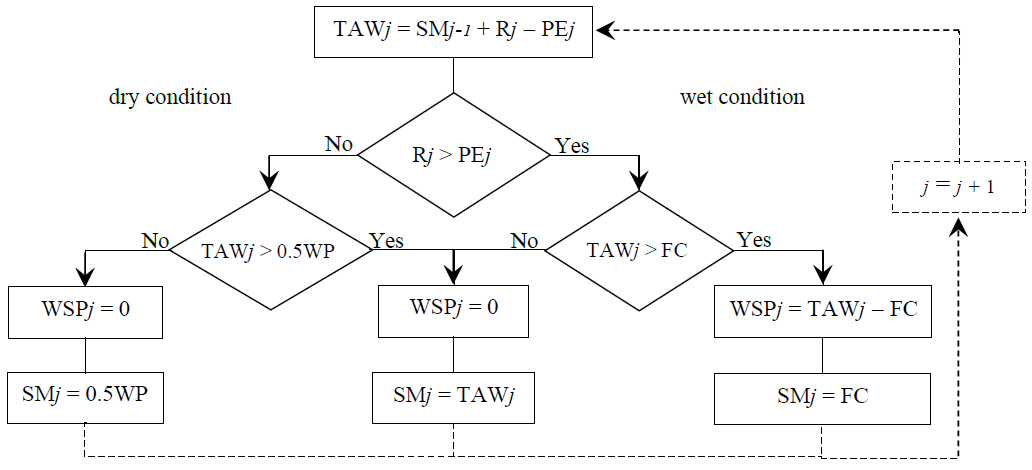
Figure 3: The model calculations flowchart Variability of the Annual Values The annual values were calculated by summing the daily water balance parameters: rainfall, pan evaporation, and the WS amount. In addition, the number of rainy days and the number of days with WS were counted for each year. The annual rainfall totals (AR) in each station were standardized as follows:
[6]
where: is the annual standard score in year y, ARy is the annual rainfall total in year y, AR is the mean annual rainfall over the study period and stdAR is the standard deviation of the series. This treatment leads to new series in which the mean equals to zero and the variance is set to 1. These values enabled the creation of a calendar for each station in which all years were divided into five categories as follows [25]: Very dry (VD) when zy < − 1.0 Dry (D) when − 1.0 ≤ zy < − 0.5 Normal (N) when − 0.5 ≤ zy ≤ 0.5 Wet (W) when 0.5 < zy ≤ 1.0 Very wet (VW) when 1.0 < zy For each parameter the mean value was calculated in each category and the ratio VW/VD was computed.
Results
Daily Scale
Table 2 presents the sorted WS probabilities at Bet Dagan station in all 56 analyzed years at this station for a sample period of 3 weeks during October and November, calculated according to Equation [5], for a soil depth = 50 mm. For example, on 22 October there was only one day of WS with 13.2 mm, therefore the probability of getting a WS amount of 13.2 mm or less, on that day, is 1.8% (1/(56+1)). On 29 October there were 4 days with WS. The probability of getting a WS amount of 30.3 mm or less, is 1.8%, 14.3 mm or less, on that day, is 3.5%, 12.2 mm or less, is 5.3% and 4.7 mm or less, the probability is 7.0%.
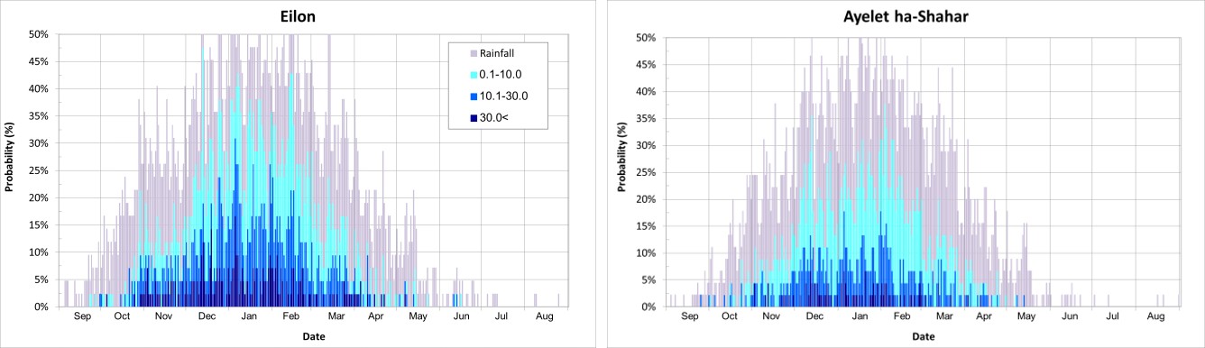
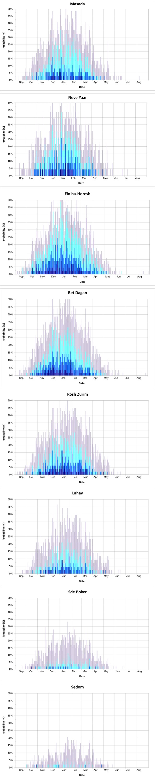
Figure 4 is an example of the annual course of the distribution of rainy days and days with WS amount divided into three groups (0.1-10.0; 10.1-30.0; >30.0), for a soil depth = 50 mm. It can be noticed that the probability for a specific day in winter months (DJF) to be a rainy day is higher than in the other seasons as expected. At the Mediterranean stations these probabilities are above 30% and at Eilon station even more than 50%. Whereas, at the arid stations, it is rare that these probabilities exceed 25%. The annual course of the probability to get a day with WS for a soil depth = 50 mm starts at most Mediterranean stations, in the first half of October and ends towards the end of April or the beginning of May. At Ein ha-Horesh station, with a Brown Red Sandy Soil, whose available water storage is relatively low (Figure 2), the probabilities are higher and the span of time when WS can be observed is longer and lasts from September to mid-May.
| Probability (%) | October | November | |||||||||||||||||||
| Probability (%) | 22 | 23 | 24 | 25 | 26 | 27 | 28 | 29 | 30 | 31 | 1 | 2 | 3 | 4 | 5 | 6 | 7 | 8 | 9 | 10 | 11 |
| 14.0 | |||||||||||||||||||||
| 12.3 | |||||||||||||||||||||
| 10.5 | |||||||||||||||||||||
| 8.8 | 0.1 | 4.7 | 2.9 | 5.5 | 1.6 | 2.1 | 12.4 | ||||||||||||||
| 7.0 | 0.6 | 1.3 | 5.3 | 4.7 | 7.0 | 5.8 | 13.1 | 3.3 | 12.9 | 1.5 | |||||||||||
| 5.3 | 1.7 | 11.0 | 7.6 | 12.2 | 8.4 | 27.3 | 7.7 | 6.6 | 2.4 | 2.6 | 15.7 | 3.3 | 15.6 | 3.6 | 7.0 | ||||||
| 3.5 | 7.3 | 10.8 | 12.9 | 2.5 | 11.6 | 9.7 | 14.3 | 1.4 | 11.9 | 8.1 | 29.3 | 29.3 | 6.7 | 6.4 | 4.1 | 24.9 | 35.2 | 20.1 | 9.9 | 18.8 | |
| 1.8 | 13.2 | 9.4 | 51.3 | 30.5 | 5.9 | 14.8 | 23.2 | 30.3 | 38.1 | 24.7 | 24.9 | 32.5 | 37.6 | 10.3 | 10.2 | 19.1 | 88.1 | 52.7 | 37.7 | 24.1 | 29.3 |
| 0.1 – 10.0 | 10.1-30.0 | >30 |
Table 3: Sorted WS amount (mm) for the dates 22 Oct – 11 Nov at Bet Dagan for soil depth = 50 mm.
At the arid stations (Sedom and Sde Boker), as expected, the WS probabilities are much lower than in the Mediterranean stations. Whereas, for example, at Bet Dagan, there are 175 days with WS amount greater than 30 mm spanning over the period 24 October to 24 March (152 days), and their probability usually does not exceed 3.5% (once every 28 years). At Sde Boker, there are only 7 days with WS amount greater than 30 mm which span from 15 October to 25 January (103 days) and their probability is 1.9% (once every 53 years).
Regarding days with WS amount less or equal 10 mm there are 815 such days (in 56 years) at Bet Dagan, spanning over a longer period, from 1 October to 7 May (219 days). There are only 23 days exceeding a probability of 25% (once every 4 years).
At Sde Boker there are 175 days such days spanning from 25 October to 29 April (187 days), Their probability usually does not exceed 4% (once every 25 years) and there is only one such day with a probability of 10% (once every 10 years).
Annual Scale
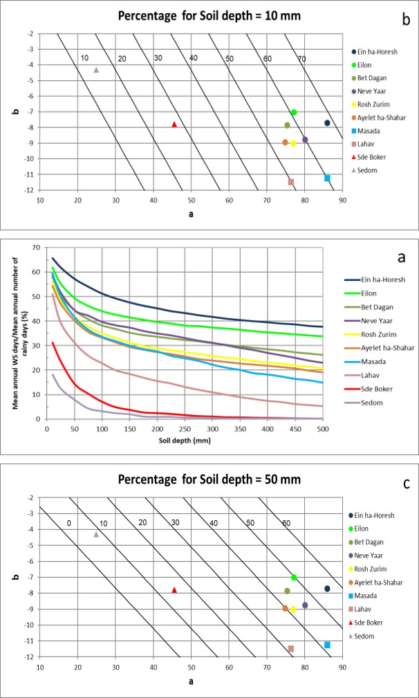
Figure 5a presents the percentage of the number of days with WS out of the total rain days. For example, at Bet Dagan, for soil depth = 10 mm, 58.1% of the rainy days produced WS. This figure decreased to 44.5% at 50 mm soil depth and decreased further to 32.3% for soil depth = 250 mm. This decrease can be best described by a logarithmic function:
Yn = a + b ln_(soil depth)_ [7]
where: Yn is the percentage of the number of days with WS out of the total rain days, a and b are the equation coefficients. Figures 5b-5d present the coefficients of the fitted logarithmic functions obtained for each station for three selected soil depths; 10, 50 and 250 mm respectively (r2 values are very high and in most stations are above 0.99). In addition, isolines of equal percentages were calculated using Equation [7].
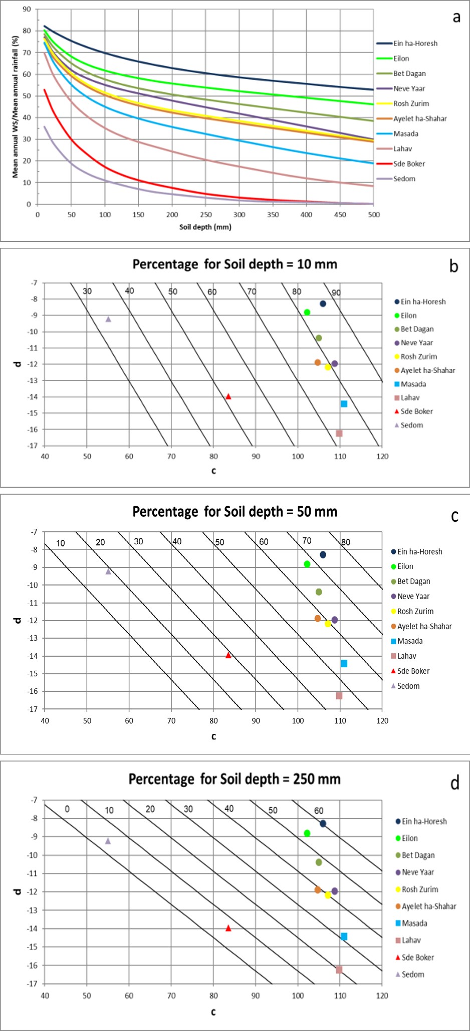
Similarly, Figure 6a presents the percentage of the mean annual WS amount (mm) out of the mean annual rainfall. For example, at Bet Dagan, for soil depth = 10 mm, 78.5% of the mean annual rainfall transformed into WS. For a soil depth of 50 mm, this percentage decreases to 65.1% and for soil depth = 250 mm the percentage decreased to 48.4%. This decrease, common to all stations, can be also best described by a logarithmic function: Ya = c + d ln_(soil depth) [8] where: _Ya is the percentage of the mean annual WS amount (mm) out of the mean annual rainfall, c and d are the equation coefficients.
Figures 6b-6d present the coefficients of the fitted logarithmic functions obtained for each station for three selected soil depths; 10, 50 and 250 mm respectively (r2 values are very high and in most stations are above 0.99). In addition, isolines of equal percentages were calculated using Equation [8].
Table 3 presents the obtained values in very dry (VD) and very wet (VW) conditions as defined in Section 2.4. While the mean annual rainfall is 1.85 times more in VW years compared to VD years at Neve Yaar (722.3 mm vs. 390.4 mm), it increased to 3.33 at Sde Boker (150.6 mm vs. 45.2 mm respectively). The ratio of the other stations is within that range, except at Sedom (arid station) where VW years compared to VD years are 14.76 (88 mm vs. 6 mm). The
ratios of the other rainfall parameters: mean annual number of rain days and mean daily intensity, which is the division the mean annual rainfall by the mean annual number, are lower than the ratio of the rainfall. Except, Sedom, the ratios of the mean annual number of rain days vary between 1.39 at Eilon (88.1 vs. 63.4) and 1.95 at Masada (76 vs. 39). The ratios of the mean daily intensity is almost the same, 1.21 at Neve Yaar (11.2 mm vs. 9.2 mm) and 2.41 at Sde Boker (4.6 mm vs. 2.2 mm). Pan evaporation values are quite uniform among the stations, and are almost the same both in VD and
VW conditions.
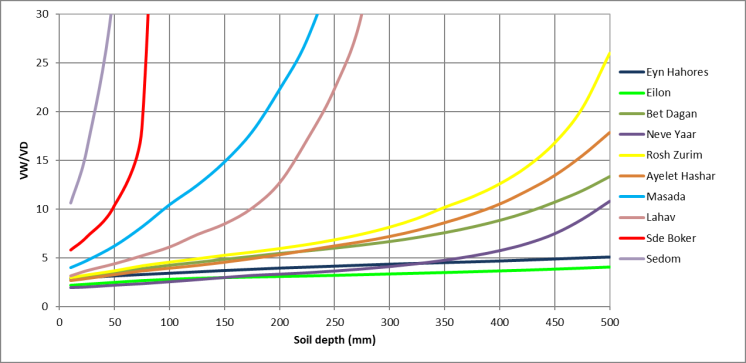
Figure 7 presents the ratio VW/VD of the mean annual WS amount for the various soil depths. It can be observed that as soil depth increases the ratio also increases, for example, at Bet Dagan station, for soil depth = 10 mm the ratio is 2.73 and increased to 3.45 when a soil depth of 50 mm is considered and increased further to 5.99 for soil depth = 250 mm. Since at Sedom station in VD years no WS was produced, the ratio VW/D is presented instead for that station.
| Mean annual rainfall (mm) | Mean annual rain days | Mean daily intensity (mm/day) | Mean pan evaporation (mm) | |||||||||
| VD | VW | Ratio | VD | VW | Ratio | VD | VW | Ratio | VD | VW | Ratio | |
| Eilon | 556.6 | 1116.0 | 2.01 | 63.4 | 88.1 | 1.39 | 8.77 | 12.66 | 1.44 | 1702.0 | 1660.5 | 0.98 |
| Ayelet ha-Shahar | 289.0 | 672.5 | 2.33 | 48.7 | 76.8 | 1.58 | 5.94 | 8.75 | 1.47 | 2009.9 | 1960.2 | 0.98 |
| Neve Yaar | 390.4 | 722.3 | 1.85 | 42.3 | 64.5 | 1.52 | 9.22 | 11.20 | 1.21 | 1700.3 | 1630.3 | 0.96 |
| Masada | 210.2 | 667.3 | 3.17 | 39.0 | 76.0 | 1.95 | 5.39 | 8.78 | 1.63 | 1797.4 | 1681.7 | 0.94 |
| Ein ha-Horesh | 345.9 | 916.8 | 2.65 | 48.8 | 74.0 | 1.52 | 7.08 | 12.39 | 1.75 | 1719.6 | 1643.1 | 0.96 |
| Bet Dagan | 351.5 | 813.1 | 2.31 | 47.4 | 66.6 | 1.40 | 7.41 | 12.20 | 1.65 | 1722.4 | 1724.7 | 1.00 |
| Rosh Zurim | 308.6 | 820.5 | 2.66 | 42.3 | 68.3 | 1.62 | 7.30 | 12.02 | 1.65 | 1807.4 | 1868.6 | 1.03 |
| Lahav | 176.7 | 449.0 | 2.54 | 33.2 | 52.3 | 1.58 | 5.33 | 8.59 | 1.61 | 1890.5 | 1829.3 | 0.97 |
| Sedom | 6.0 | 88.0 | 14.76 | 4.8 | 20.1 | 4.19 | 1.24 | 4.37 | 3.52 | 3857.0 | 3669.5 | 0.95 |
| Sde Boker | 45.2 | 150.6 | 3.33 | 21.0 | 32.8 | 1.56 | 2.15 | 4.60 | 2.14 | 2411.6 | 2313.8 | 0.96 |
Table 4: Comparison between very dry (VD) and very wet (VW) conditions.
Discussion
In the current water balance approach, water surplus is assumed to occur on days when the rainfall is greater than the potential evaporation and the soil moisture reaches FC (wet conditions on Figure 3). Consequently, water surplus equals to the quantity of water in excess of that required to bring the soil to FC. During most of the dry season no evaporation actually occurs and thus the soil moisture (SMj), is set to the minimum possible value - 0.5WP (dry conditions on Figure 3).
The presented distributions in Figure 4 enable evaluation of the probability of any day during the year to be rainy and the probability that this day will have WS and its amount. It is more detailed than weekly (and monthly) time steps [26], monthly [27] or annual values [28, 29]. Figure 4 highlights also the advantage of this presentation for agricultural and ecological applications, as it can be used to predict plant growth period and it enables identification of risks to the plant at various growth stages. In addition, the temporal distribution of the WS and the rainfall may be used for evaluating the timing of occurrence of geomorphological and hydrological processes, such as runoff, stream flow and level of groundwater and lakes.
Since the model calculates the WS for each day, the summation of the amount and the number of days provides a general view of the hydrological conditions of the different stations. The probabilistic representation of the results (Figures 5 and 6) enables a comparison among stations with different rainfall regimes and soil types. It can be noticed that the a coefficients of the fitted functions in Figure 5b-5d (presenting the percentage of the number of days with WS out of the total rain days) are similar for all Mediterranean and Semi-Arid climate stations regardless of their annual rainfall total (ranging from 300 to 800 mm). These coefficients range between 75 and 86. However, they decrease a great deal in the arid region, 46 in Sde Boker (92.9 mm) and 25 in Sedom (40.6 mm), (Figures 5b-5d).
It should be emphasized that the location of the various dots in Figures 5b-5d (each representing a different station) remain at the same place on the chart regardless of the selected soil depth. The only thing that varies are the orientation of the lines which in turn define the percentages. Thus, for example, it can be noticed that the percentage of WS days for soil depth=10 mm in Masada is higher than that for Rosh Zurim and Ayelet ha-Shahar (60% vs. 55% and 56% respectively, Figure 5b), almost equal for soil depth=50 mm (40% in Ayelet ha-Shahar, 42% in the other two, Figure 5c) and lower for soil depth=250 mm (25% in Masada, 26% in Ayelet ha-Shahar and 27% at Rosh Zurim, Figure 5d).
Very similar results were obtained also with the c coefficients of the fitted functions in Figure 6a (presenting the percentage of the mean annual WS (mm) out of the mean annual rainfall). In the Mediterranean and Semi-Arid climate region they range between 102 and 111, whereas in the arid region they decrease to 84 and 55 in Sde Boker and Sedom respectively. Here again the differences between stations can be noticed as soil depth varies. For example, the percentage of WS amount for soil depth=10 mm in Eilon, Bet Dagan and Neve Yaar are very similar (80%, 79% and 77% respectively, Figure 6b). For soil depth=50 mm the differences among these stations increase (68%, 65% and 62% respectively, Figure 6c). Finally, at a soil depth of 250 mm, the differences are considerable (54%, 48% and 45% respectively, Figure 6d).
A comparison between the percentage of the number of days with WS (Figure 5a) and the percentage of the WS amount (Figure 6a) shows that at all stations for all soil depths the percentage of WS amount is higher than the percentage of WS number. This is due to the fact that daily rainfall amounts are very positively skewed in all the Mediterranean region (e.g. Reiser and Kutiel [30]). In other words, there are many rain days with minute amounts that do not contribute very much to the annual total and certainly do not produce any WS but increase considerably their number, whereas, there are few rain days with considerable amounts that are responsible for most of the WS. Thus, when the total number of rain days with WS is calculated out of the total rainy days, their percentage is relatively low. On the other hand, the accumulated rainfall during the very rainy days, are responsible for the majority of the WS amount and therefore their percentage is higher. For example, at Bet Dagan at soil depth = 50 mm the mean annual WS days represent 44.5% of the mean annual rain days (25.9 out of 58), (Table 1) whereas, the mean annual WS amount is 355.6 mm out of 545.8 mm mean annual rainfall totals meaning 65.1%.
Comparison was made with two other regions. The first is Lake Pontchartrain basin, Louisiana, USA [27], a humid subtropical climate, where the mean annual rainfall is between 1600 mm and 1723 mm and the mean annual WS is between 666 mm and 737 mm (for soil moisture capacity of 150 mm which represent 1000 mm soil depth). Thus, on average the percentage of the mean annual WS (mm) out of the mean annual rainfall is 42.7%. The second region is Salado river basin, Buenos Aires province, Argentina [29], a temperate and humid climate, where the mean annual rainfall is between 800 mm and 1000 mm and the mean annual WS is between 146 mm and 223 mm (soil depth was not mentioned). Thus, the percentage of the mean annual WS (mm) out of the mean annual rainfall is about 20%.
The division of the years into five categories enables a better insight of the inter-annual variability of the water balance parameters. At most stations, the mean annual rainfall is more than double in VW years compared to VD years (Table 3). This increase in the annual rainfall is due to an increase of the mean annual number of rain days and their mean daily intensity in VW years as compared to VD years. However, their importance is not equal. At Ayelet ha-Shahar, Neve Yaar, Masada and Sedom the ratios of the mean annual number of rain days are higher than the ratios of the mean daily intensity. At the other stations, the ratios of the mean daily intensity are higher. Table 3 shows, also, a minor variation in pan evaporation between VW and VD years, which indicates an almost uniform evaporation during the rainy season meaning that the fluctuations occur mainly during the dry season. Finally, the ratio VW/VD of the mean annual WS amount increases as soil depth increases (Figure 7). This follows the relatively low values of WS amount in VD years, resulting in high ratios. For example, at Bet Dagan, for soil depth = 10 mm 697.8 mm vs. 264.6 mm and the ratio is 2.73, for soil depth = 100 mm in VW years it decreased to 564.4 mm vs. 133.1 mm and the ratio increased to 4.24. At Lahav, for soil depth = 10 the WS amount are lower and in VW years is mm 339.5 mm vs. 108.2 mm and the ratio is 3.14, for soil depth = 100 mm 220.7 mm vs. 36.1 mm and the ratio is 6.11. Since, WS amount decreases as aridity increases resulting in increasing ratios accordingly. Three groups of stations can be distinguished in the figure according to their climatic region: Mediterranean, Semi-Arid and Arid climates.
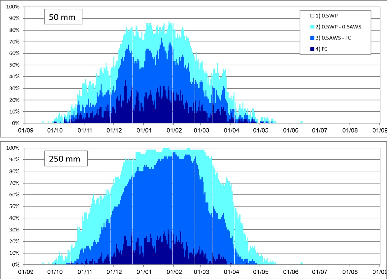
Apart from water surplus, the daily soil moisture is also a product of the model (Equation 2). Figure 8 presents an example of the annual course of the distribution of SM at Bet Dagan for two soil depths; 50 and 250 mm for 4 water storage capacities: (1) 0.5WP (the white area); (2) from 0.5WP to 0.5AWS; (3) from 0.5AWS to FC; and (4) FC. As expected, the probabilities for the various SM levels follow the daily rainfall pattern (see Figure 4). Since the available water storage increases with increasing soil depth (Figure 2), there are differences in the SM distributions, among SM groups and within each SM group. For example, at soil depth = 50 mm with SM content of FC, it starts at the beginning of October and ends towards the beginning of May (219 days) and the probabilities usually does not exceed 25% with peaks up to 40%. For a soil depth = 250 mm, it is a shorter period, from mid-October to the end of March (170 days), and the probabilities usually does not exceed 20%. In addition, soil depth sensitivity to evaporation, decreases with increasing depth [31, 32], as a result the probabilities for SM of soil depth = 50 mm are much lower than for soil depth = 250 mm. For example, for SM 0.5WP to 0.5AWS (group 2), the probabilities at soil depth = 50 mm are around 75% with peaks up to 85%. At soil depth = 250 mm, for the same SM level, these probabilities are above 90%. Moreover, for SM 0.5AWS to FC (group 3) at soil depth = 50 mm there are 92 days at the probability = 50% compared to 148 days at soil depth = 250 mm. Figure 8, emphasizes also, that in the Mediterranean climate most of the time no evaporation actually occurs and the SM is at 0.5WP (the white area).
The presented water balance model has dynamic components, which are the observation series of both daily rainfall and daily pan evaporation, and less dynamic components like soil properties which are expressed by the water holding capacity for a given depth. The only parameter that needs to be estimated is the soil depth, all the others are published measured data. This study did not set a priori value of soil depth, but rather considered a range of 21 possible depths to simulate a variety of root zone depths.
In humid regions runoff is generated by saturation excess (Dunne mechanism), while in arid and semi-arid regions and part of the Mediterranean regions infiltration excess (Hortonian mechanism) dominates. Therefore, in most of the research stations runoff is generated when the rainfall intensity exceeds the infiltration capacity of the upper soil (sometimes with presence of crust) even before the root zone depth reaches FC [33, 34]. It appears that the depth parameter in the model in such regions should be set to a smaller value than the actual root zone depth.
Summary and Conclusions
The annual course of the distribution of days with water surplus was estimated by a simple water balance model, which combines daily rainfall data and daily pan evaporation with soil water properties. Water surplus is the fraction of precipitation which does not evaporate and is not stored in the soil storage and includes both surface runoff and deep percolation. The above model was run using available published daily rainfall series and daily pan evaporation from ten Israel Meteorological Service stations, representing the various climatic conditions in Israel and by using a range of 21 possible depths to simulate a variety of root zone depths.
In addition, the summation of the water surplus amount and the number of days with surplus water provides a general view of the hydrological conditions of the different stations. The probabilistic representation of the results enables a comparison among stations with different rainfall regimes and soil types.
The inter-annual variability of the water balance parameters was analyzed by division the years into five categories. The differences between wet and dry conditions can be used as effective tool to compare between the water balance parameters in the various climatic regions.
The model does not contain coefficients or complex parameters; the only parameter that needs to be estimated is the soil depth.
This simple daily model ignores phenomena associated with frozen water such as snowfall and snowmelt (which are rare in Mediterranean, semi-arid or arid regions) and can be applied to other regions with similar conditions, without any special adjustment.
The presented model enables evaluation of the probability that each day of the year will have water surplus and its amount and can be input to various hydrological models and an important tool for the planner. In addition, this information can be used to predict plant growth period and it enables identification of risks to the plant at various growth stages, and also enable evaluating the timing of occurrence of geomorphological and hydrological processes which depend, for example, on the water surplus in different seasons during the year.
Acknowledgments
The authors wish to thank Ms. Noga Yoselevich for her excellent help with preparing the figures.
References
-
Thornthwaite CW (1948) An approach toward a rational classification of climate. Geographical Review 38(1): 55- 94.
-
Thornthwaite CW, Mather JR (1955) The water balance. Publication in Climatology 8(1): 1-104.
-
Thornthwaite CW, Mather JR (1957) Instructions and tables for computing potential evapotranspiration and the water balance. Publication in Climatology 10(3): 185-311.
-
Budyko MI (1974) Climate and life. Academic Press, New York, pp: 508.
-
Eagleson PS (1978) Climate, soil and vegetation: 1. Introduction to water balance dynamics. Water Resources Research 14(5): 705-712.
-
Milly PCD (1994) Climate, soil water storage, and the average annual water balance. Water Resources Research 30(7): 2143-2156.
-
Scotter DR, Clothier BE, Turner MA (1979) The soil water balance in a Fragiaqualf and its effect on pasture growth in Central New Zealand. Australian Journal of Soil Research 17(3): 455-465.
-
Sophocleous MA (1991) Combining the soilwater balance and water-level fluctuation methods to estimate natural groundwater recharge: practical aspects. Journal of Hydrology 124(3-4): 229-241.
-
Rushton KR, Ward C (1979) The estimation of groundwater recharge. Journal of Hydrology 41(3-4): 345-361.
-
White RE, Helyar KR, Ridley AM, Chen D, Heng LK, et al. (2000) Soil factors affecting the sustainability and productivity of perennial and annual pastures in the high rainfall zone of south-eastern Australia. Australian Journal of Experimental Agriculture 40: 267-283.
-
Walker GR, Zhang L (2002) Plot-scale models and their application to recharge studies. In: _Studies in catchment_ _hydrology: the basics of recharge and discharge_. Edited by Zhang, L. and G.R. Walker, CSIRO Publishing, Australia.
-
Zhang L, Walker GR, Dawes WR (2002) Water balance modelling: concepts and applications. In: _Regional water_ _and soil assessment for managing sustainable agriculture_ _in China and Australia_. Edited by McVicar, T.R., L. Rui, J. Walker, R.W. Fitzpatrick, and L. Changming. ACIAR Monograph 84: 31-47.
-
Perrin C, Michel C, Andreassian V (2001) Does a large number of parameters enhance model performance? Comparative assessment of common catchment model structures on 429 catchments. Journal of Hydrology 242(3-4): 275-301.
-
Reiser H, Kutiel H (2009) Rainfall uncertainty in the Mediterranean: definitions of the daily rainfall threshold (DRT) and the rainy season length (RSL). Theoretical and Applied Climatology 97: 151-162.
-
Reiser H, Kutiel H (2010) Rainfall uncertainty in the Mediterranean: Intraseasonal rainfall distribution. Theoretical and Applied Climatology 100: 105-121.
-
Richter DD, Markewitz D (1995) How deep is soil? BioScience 45(9): 600-609.
-
Kuriakose SL, Devkota S, Rossiter DG, Jetten VG (2009) Prediction of soil depth using environmental variables in an anthropogenic landscape, a case study in the Western Ghats of Kerala, India. Catena 79(1): 27-38.
-
Mehnatkesh A, Ayoubi S, Jalalian A, Sahrawat KL (2013) Relationships between soil depth and terrain attributes in a semi arid hilly region in western Iran. Journal of Mountain Science 10(1): 163-172.
-
Ravikovitch S (1981) _The Soils of Israel: Formation,_ _Nature and Properties_. Hakibbutz Hameuchad Publishing House, Tel-Aviv.
-
Canadell J, Zedler PH (1995) Underground structures of woody plants in Mediterranean ecosystems of Australia, California and Chile. In: _Ecology and biogeography_ _of Mediterranean ecosystems in Chile, California and_ _Australia_. Edited by Arroyo, M.T.K., Zedler, P.H. and M.D. Fox. Springer-Verlag, New-York, pp: 177-210.
-
Hillel D (1971) _Soil and Water_. Academic Press, New York & London.
-
Rushton KR, Eilers VHM, Carter RC (2006) Improved soil moisture balance methodology for recharge estimation. Journal of Hydrology 318(1-4): 379-399.
-
Penman HL (1948) Natural evaporation from open water, bare soil and grass. Proceedings of the Royal Society of London Series A 193(1032): 120-145.
-
Stanhill G (1961) A comparison of methods of calculating potential evapotranspiration from climatic data. Israel Journal of Agricultural Research 11: 159-171.
-
Kutiel H, Salinger J, Kingston DG (2020) Spatial and temporal characteristics of rain-spells in New Zealand. Theoretical and Applied Climatology 142: 329-348.
-
Srinivas S, Srinivas CV, Nair KM, Naidu LGK, Dipak Sarkar, et al. (2016) A climatic water balance model ‘WatBal’ for bioclimatic classification and agroclimatic analysis. Ecology, Environment and Conservation 22(1): 173-180.
-
Rohli RV, Grymes JM (1995) Differences between Modeled Surplus and USGS-Measured Discharge in Lake Pontchartrain Basin, Louisiana. Water Resources Bulletin 31(1): 97-107.
-
Crapper PF, Fleming PM, Kalmab JD (1996) Prediction of lake levels using water balance models. Environmental Software 11(4): 251-258.
-
Scarpati OE, Spescha LB, Lay JAF, Capriolo AD (2011) Soil water surplus in Salado river basin and its variability during the last forty years (Buenos Aires Province, Argentina). Water 3(1): 132-145.
-
Reiser H, Kutiel H (2012) The dependence of the annual total on the number of rain-spells and their yield in the Mediterranean. Geografiska Annaler 94(3): 285-299.
-
Milly PCD, Dunne KA (1994) Sensitivity of the global water cycle to the water-holding capacity of land. Journal of Climate 7(4): 506-526.
-
Wu W, Geller MA, Dickinson RE (2002) The Response of Soil Moisture to Long-Term Variability of Precipitation. Journal of Hydrometeorology 3(5): 604-613.
-
Hillel D, Tadmor N (1962) Water regime and vegetation in the central Negev highlands of Israel. Ecology 43(1): 33-41.
-
Farmer D, Sivapalan M, Jothityangkoon C (2003) Climate, soil, and vegetation controls upon the variability of water balance in temperate and semiarid landscape: Downward approach to water balance analysis. Water Resources Research 39(2): 1035.
- Lessons to Learn: Trees are More than the Lungs of the World
- Community Forestry Enterprises as a Model for Sustainable Forest Development: The Case Of The "Baja Tarahumara" in Chihuahua, Mexico
- Ecological and Socio-Economic Impacts of Chromolaena odorata and Mesosphaerum suaveolens, Two Invasive Alien Species in Central and Southern Benin, West Africa
- Epigenetic Sustainability: Modeling the Human Factor as a Natural Resource through Science 4.0 and the NR3C1 Biological Pilot
- Growth-at-Risk: A Framework for Assessing Economic Vulnerability
- The Rural Territory as a Socioecological System for the Management of Public Policy for Sustainable Rural Development