On the Understanding of Time in the Real World, and in the World of Computing

Outline

1. Introduction
2. Atom clocks, Sommerfeld’s Fine-Structure Constant and Koltsov’s Zero Point Fluctuations (ZPFs)
3. The Meaning of the Use of Legendre transformation and Hamiltonian in Modern Hopfield Networks
4. The Concept of ‘Time Islands’ in DNA and the Propagation of an Intrinsic Perturbation along the DNA axis
5. Biological Feedback Loops as ‘macroscopic’ Time Islands of the Organism

6. Large Scale Eddies and Time Islands in Climate Modeling and Meteorology 7. Concluding Remarks “Close your eyes”, the yoga instructor said, “there is no past, no future, only the moment of now. Imagine…”. While following my breath, I realize that also no counting is possible, when only this moment of now exists. Therefore, mindless ‘counting’ belongs to a different world… (personal reflections, unpublished).

Introduction

“Time is impenetrability”, Alan Turing said, with a tacit smile to Humpty Dumpty and Alice [1], rendering time to the mysterious. “The Times they are a-changing”, the bard sang, making it plural, perennially. In Greek mythology, and in pre-Socratic philosophy, ‘Time’ was personified in the god Chronos. In antiquity, and in Renaissance literature based hereupon, Chronos’ name became intermingled with Cronus, the Titan who devoured his children. But eventually the Titans were defeated in a heroic battle.

“Space is emergent, and gravity is emergent, but there should be Time. Time is needed, fundamentally, because dynamics are needed”, the modern physicist says [2]. In the word ‘need’ an essential key is hidden: the key of purpose, the unspoken reason why so much effort is invested in understanding, comprehending, and also the desire of controlling the nature of things, Time being the ultimate ‘thing’.

The philosophical antithesis between ‘time as duration’, following Henri Bergson (1859-1941) [3, 4], and time as an abstract dimension of four-dimensional Minkowski spacetime, following Hermann Minkowski (1864-1909) [5], has been overstepped by theories claiming that time corresponds to ‘time intervals’ that can be measured by clocks [6, 7]. This philosophical dichotomy however became fruitful in analyzing the role of a comprehension of the notion of time in various fields of contemporary science and culture, from the fine structure of matter to the understanding of global weather systems and the climate. And even so it happened in the mathematical undergirding of AI through the construction of Modern Hopfield Network learning in AI algorithms (see ¶3). Based on the property of stable time intervals, among other considerations, the International System of Units (SI) has defined the second, the SI-unit of time, “as the fixed numerical value of the cesium frequency $\Delta v_{cs}$, being the unperturbed ground-state hyperfine transition frequency of the cesium-133 atom, to be 9192631770 when expressed in the unit Herz (Hz), which is equal to $s^*$” [8] see ¶2).

According to Koltsov [7, 9] a more general definition of time is inferred from the intensity of so-called zero-point fluctuations of the electromagnetic field (ZPFs) in metals (see ¶2). Moreover, these ZPFs can also be developed into a relativistic relationship between material objects, consistent with the Lorentz transformation of time when approximating the universal speed of light (c), after Hendrik A. Lorentz (1853-1928) [10, 11]. The Lorentz transformation of time is represented by the formula:

$$t' = \frac{1 - \frac{v}{c}}{1 - \frac{v^2}{c^2}}$$

which in fact is a physical law defining the invariance of the speed of light (c) in vacuum, with $t$ and $v$ the time, resp. velocity in coordinate system 1, and $t'$, $v'$ in a second coordinate system linearly displaced according to system 1.

In section ¶2, we will elaborate on Koltsov’s theory [7, 9], showing that Koltsov builds upon the observation of a “slowdown of spontaneous low-energy EM transitions in atomic nuclei when they are placed into metal matrices”, which is consistent with Sommerfeld’s finding of the dimensionless fine-structure constant [12]. Moreover, in Koltsov’s paper, the number of quanta of ZPFs interacting with any particle in a single frequency interval is also a constant, so the number of ZPFs does not depend on the ZPF’s frequency [7].

Both in Koltsov’s theory and in the unrelated theory of modern Hopfield networks [13] used for dense associative learning algorithms (and their use in AI), an important role is played by the mathematical technique of the Legendre transformation of continuous functions, in particular the Lagrangian ($^*1$), which is best known among physicists as the Hamiltonian. In section ¶3, we will come back to the conceptual link and formal parallelism between Hopfield network computing and Quantum physics, which also was applied to spin magnetic fields. An example of the latter is found in Glauber dynamics (i.e. an Ising model evolving in time) used to describe the thermal equilibrium of the sin-spin interactions in magnetism [14]. In mathematical optimization, the method of Lagrange multipliers is a strategy for finding the local maxima and minima of a function subject to equation constraints (i.e. subject to the condition that one or more equations have to be satisfied exactly by the chosen values of the variables [15].

Moreover, it appears that the Hamiltonian (see section ¶3.) has been particularly useful in quantum-mechanic systems where the Hamiltonian is explicitly time-independent. On the other hand, several examples in this paper are drawn from the fields of biology, meteorology and climate-modeling where the notion of time-interval has been constructed independently from quantum-mechanical considerations (Sections ¶4-6). In particular, the influence

1 The Lagrangian operator is a well-known notion in physics to describe the conservation of the energy of a system. It is represented by the function $L$ within a configuration space $M$, that for many systems is given by the formula $L = T-V$, where $T$ and $V$ are the kinetic, resp. potential energy of the system (see also section ¶3. of this paper).

of DNA-content on the propagation characteristics of an intrinsic perturbation along the DNA-axis [16, 17] shows the influence of emergent realms of nature on the working of ‘Time’, designated as ‘Time-islands’ (see section ¶4). Further, other analogies are explored such as found in the life sciences and also in meteorology, in order to get a better grip on the nature of time and its characteristics. Or, in other words, if the reduction of all knowledge to the dynamics of physics belongs to the beyond-physical notion of Time (*²*), then this reduction becomes senseless, when emergent realms indicate an intrinsic dependency of time. However, what does this implicate for the reduction of all knowledge to the time-independent algorithms of computing and AI, or, how is time materialized in the world of computing?

It appears that the modern ambitions of taming the ‘titan’ (like Cronos), by reducing or obliterating it, somehow have brought it back. Are we consumed by Time, or devoured by it? Or, can we hear the alternative, our being in time, harmoniously expressed in numerous aspects of life as well as in the immaterial objects surrounding us, from the smallest particles to the movements in our solar system?

Atom clocks, Sommerfeld’s Fine-Structure Constant and Koltsov’s Zero Point Fluctuations (ZPFs)

In the relativistic physics of describing motion in different, linearly displaced coordinate frames, it was important to have formulas to express and measure the simultaneity of events, for various reasons. Primarily, this follows from the prohibition in the real world to go backwards in time [18], and concomitantly, the impossibility to surpass the speed of light (in vacuum). Despite the reversibility of time in quantum physics, such as in the definition of positrons (antimatter) as being equal to “electrons propagating backwards in time” (see e.g. the Feynman diagrams after Richard P. Feynman [1918, 1919, 1920, 1921, 1922, 1923, 1924, 1925, 1926, 1927, 1928, 1929, 1930, 1931, 1932, 1933, 1934, 1935, 1936, 1937, 1938, 1939, 1940, 1941, 1942, 1943, 1944, 1945, 1946, 1947, 1948, 1949, 1950, 1951, 1952, 1953, 1954, 1955, 1956, 1957, 1958, 1959, 1960, 1961, 1962, 1963, 1964, 1965, 1966, 1967, 1968, 1969, 1970, 1971, 1972, 1973, 1974, 1975, 1976, 1977, 1978, 1979, 1980, 1981, 1982, 1983, 1984, 1985, 1986, 1987, 1988]) [19], in most (of the macroscopic) applications in the real world, the irreversibility of time is considered mandatory.

The necessity of finding a hyper-stable unit of time interval as reference system for measuring universal time, has led to the technological construction of a number of time reference systems of which the SI definition of the second has already been recalled in the introduction (see ¶1). The global/Greenwich time and the global positioning system (GPS), the latter derived from the US Department of Defense [20], are equally well-known examples. Whereas in a different, philosophical approach of ‘time as duration’ [3, 4], the simultaneity of different events (e.g. acoustic and visual signals) perceived by an individual is considered instrumental to the notion of simultaneity (e.g. during listening to music), such simultaneity neither of events nor of personal perceptions is required in a technological approach of ‘measurable time’ [4]. And even the integrity of human perceptive skills is no longer considered helpful, like in the prophecies of David R. Priestland [21], and, most obviously, since the dehumanization of human culture has become fact [22].

The stability of atom clocks, like that based on the ground-state of the cesium-133 atom [8], has been instrumental for the working of the GPS system too. In Koltsov’s theory (see below), the frequency of spontaneous electromagnetic transitions and so-called ZPFs is found instrumental to the definition and understanding of the nature of time [7, 9]. Koltsov’s theory recalls an analogy with Arnold Sommerfeld’s (1868-1951) theory regarding the strength of interactions between elementary charged particles. Sommerfeld introduced the so-called fine-structure constant ($\alpha$) in 1916 [12] as a dimensionless quantity (or physical constant) independent of the system of units used. The formula was given as:

$$\alpha = \frac{e^2}{2\varepsilon_0 hc} = \frac{e^2}{4\pi\varepsilon_0 \hbar c} \approx \frac{1}{137}$$

with $e$ the elementary charge (1,602177634.10$^{-19}$ C), $\varepsilon_0$ the electric constant or vacuum permittivity (8,8541878188.10$^{-12}$ Fm$^{-1}$), $c$ the speed of light, $h$ the Planck constant or $h=h/2\pi$ the reduced Planck constant. In the (electrostatic) CGS (centimeter – gram – second) system of units, which sets $\varepsilon_0=c=h=1$, the formula for $\alpha$ is a bit simplified, namely

$$\alpha = e^2 / 4\pi$$

and in the system of atomic units, setting $e=h=4\pi\varepsilon_0=1$, the expression ultimately becomes $\alpha=1/c$.

Several interpretations for the physical meaning of this fine-structure constant (also named the Sommerfeld constant) have been followed, such as the ratio of the energy needed to overcome the electrostatic repulsion between two electrons (separated a distance $d$ apart) and the energy of a single photon of wavelength $\lambda=2\pi d$. (*³*)

For some simple reduction shows:

$$\alpha = \frac{e^2}{4\pi\varepsilon_0 d} \left( \frac{hc}{\lambda} \right) = \frac{e^2}{4\pi\varepsilon_0 d} \left( \frac{2\pi d}{hc} \right) = \frac{e^2}{4\pi\varepsilon_0 d} \left( \frac{d}{hc} \right) = \frac{e^2}{4\pi\varepsilon_0 hc}$$

Alternatively, the fine-structure constant $\alpha$ may be regarded as “the ratio of the velocity of the electron in the first circular orbit of the Bohr model of the atom”, being $e^2/4\pi\varepsilon_0 h$ to the speed of light in vacuum ($c$); or, the square root of the ratio of “the potential energy of the electron in the first circular orbit of the Bohr model of the atom and the energy mec2 equivalent to the mass of an electron” (*3).

Although the physical interpretations listed above are not making use of the quantum mechanical approach of matter, or may even not be (entirely) consistent with Feynman’s quantum electrodynamics (QED) [23], for an introductory reading it is convenient to say that Sommerfeld’s constant α is directly related to the coupling constant “determining the strength of the interaction between electrons and photons” [24]. This theory however doesn’t predict the value of α, and therefore, α must be determined experimentally [24].

In the theory of Koltsov [7], it is suggested that it is “the interaction of ZPFs with charged particles that leads to their quantum properties”. The reality of the existence of these ZPFs is confirmed e.g. by the Casimir effect (after Hendrik Casimir [1909, 1910, 1911, 1912, 1913, 1914, 1915, 1916, 1917, 1918, 1919, 1920, 1921, 1922, 1923, 1924, 1925, 1926, 1927, 1928, 1929, 1930, 1931, 1932, 1933, 1934, 1935, 1936, 1937, 1938, 1939, 1940, 1941, 1942, 1943, 1944, 1945, 1946, 1947, 1948, 1949, 1950, 1951, 1952, 1953, 1954, 1955, 1956, 1957, 1958, 1959, 1960, 1961, 1962, 1963, 1964, 1965, 1966, 1967, 1968, 1969, 1970, 1971, 1972, 1973, 1974, 1975, 1976, 1977, 1978, 1979, 1980, 1981, 1982, 1983, 1984, 1985, 1986, 1987, 1988, 1989, 1990, 1991, 1992, 1993, 1994, 1995, 1996, 1997, 1998, 1999, 2000]), which is defined as the “physical force acting on the macroscopic boundaries of a confined space, which arises from the quantum fluctuations of a field”(*4). For instance, inside a cavity with metal walls “there are no EM waves with lengths greater than the size of the cavity, and the pressure on the walls from ZPFs from the outside is greater than their pressure from the inside” [7].

For Koltsov [7], the value of the fine structure constant α = e2/ ћc is given by the ZPF intensity, or “the number of ZPFs quanta in a unit frequency interval passing through each space point per unit time (nZPF)”, whereby nZPF ~ 1 / π [7]. This brings Koltsov [7] to the following estimate of α and e2, being e2 ≈ ћc nZPF /32 . Moreover, “this result satisfies the requirement for a closed theory of particle interactions, in which the dimensionless interaction constant α must be calculated based on the main parameters of the theory, and not just measured in the experiment” (Koltsov, p. 3).

Whether or not Koltsov is right in his conclusion that “measuring time may be reduced to calculating the number of ZPFs” (p. 5) – based on the universality of his definition of time in free space – his theory of ZPFs, as well as the historic theories of Sommerfeld and Schott (*5) [25], point towards an intrinsic relationship between time and fine-structure of

3 According to the ‘virial theorem’ in the Bohr model of the atom (after Niels Bohr [1885, 1886, 1887, 1888, 1889, 1890, 1891, 1892, 1893, 1894, 1895, 1896, 1897, 1898, 1899, 1900, 1901, 1902, 1903, 1904, 1905, 1906, 1907, 1908, 1909, 1910, 1911, 1912, 1913, 1914, 1915, 1916, 1917, 1918, 1919, 1920, 1921, 1922, 1923, 1924, 1925, 1926, 1927, 1928, 1929, 1930, 1931, 1932, 1933, 1934, 1935, 1936, 1937, 1938, 1939, 1940, 1941, 1942, 1943, 1944, 1945, 1946, 1947, 1948, 1949, 1950, 1951, 1952, 1953, 1954, 1955, 1956, 1957, 1958, 1959, 1960, 1961, 1962]), it is stated that Uel = 2 Ukin ↔ Uel = meve 2 = me (αc)2 = α2(mec2) and Uel/mec2 = α2. From this, the velocity of an electron follows ve = αc . This quote - as well as the previous quotes on the interpretation of Sommerfeld’s constant - are from Wikipedia’s page on the ‘fine-structure constant’ (2025). (accessed: 17-07-2025).

4 See e.g. Wikipedia (2025). Casimir effect. (https://Wikipedia.org/ ) (ac- cessed: 13-08-2025)

5 See e.g. the analogy with G. Schott’s (25) proof for the relation between the “homogenously electrified sphere, with an uniformly moving center de- scribing an orbit with period T, which is non-radiating and giving only a static electric field outside the ball, when it is a whole multiple of cT/2 (with c the light speed), or b = l.cT/2 with l an integer number” (fide B. Hoenders, 2013).

matter, which however shouldn’t be regarded as indicating a contradiction with QED [26].

Last but not least, the most renowned formula of physics E= mc2, ascribed to Albert Einstein (1879 - 1955), links the mass (m) of an object to its energy (E). Einstein published his findings in one of his three famous papers of 1905, the so- called annis mirabilis [27]. According to the formula above, describing the equivalence between mass and energy, all massive objects have an intrinsic energy, even when they are in a stationary state. Alternatively formulated, “in a reference frame where the system is moving, the relativistic energy and relativistic mass (instead of rest mass) obey the same formula”. For moving objects or particles, however, the kinetic energy is given by their momentum (p), or p = mv, and, since Einstein’s mass-energy equivalence, also by a term for the relativistic mass. For massless particles such as photons, the Planck-Einstein relation is given by the equation E = hf, with h the Planck constant (see above) and f the photon frequency. Also for massless particles, the frequency, and thus the relativistic energy, are frame-independent. Since the formulation of Einstein’s mass-energy equivalence, it became common knowledge (to a degree it became an inscription on merchandise stuff, coffee mugs, T-shirts, and the like..) that eventually, in nuclear fission reactions, mass may become transformed into gigantic amounts of radiative and thermal energy, the devastative power of which are never to forget.

In a following paragraph (¶ 3.) we will expand on how the notion of time, or the dependency of time, disappears in the Lagrangian expression for describing the energy of a system in terms of their potential and kinetic energies (see also *1).

The Meaning of the Use of Legendre transformation and Hamiltonian in Modern Hopfield Networks

“Think, also, of the ladies of the land weaving toilet cushions against the last day, not to betray too green an interest in their fates! As if you could kill time without injuring eternity”. From: Henry David Thoreau, in Walden (1854), For the unexperienced, interested layman it is a surprising discovery that the same mathematical techniques paved the way to both quantum mechanics (QM) and Modern Hopfield Networks (MHN), and hence, also to the fast developments in (the theory of) AI networks. But when these developments are regarded from an eagle’s perspective, the fact that both developments (in QM and in MHN) use the formalism of minimalizing the underlying energy function in dynamical trajectories (or preserving the stability of intermediate states in a trajectory), then, the analogies appear not so surprising anymore.

The technique of Legendre transformation, after the French mathematician Adrien-Marie Legendre (1752-1833), who introduced the technique in 1787 [28]– two years before the French Revolution ! – when studying the ‘minimal surface problem’. Together with another French mathematician, Joseph-Louis Lagrange (1736-1813), who published the first part of his grand opus in 1788 [29], they provided the basis and simplified the analysis of many problems in (classical) mechanics. The Lagrangian operator still is widely used to describe the function L within a configuration space M, that for many systems is given by L= T – V, where T and V are the kinetic and potential energy of the system, respectively.

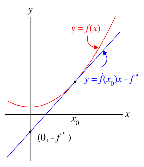
The Legendre transformation of a real-valued multivariate convex function f: I → ℜ on the interval I ⊂ ℜ is the function f*: I* → ℜ , defined by f* (s) = sup x∈ I (s x – f(x)) with domain I* = { s ∈ ℜ : sup x∈ I (s x – f(x)) < ∞ } . When f is strictly convex, meaning that all values of the function on the interval [x, y] between x and y are below the values of the line between f(x) and f(y), then the supremum norm can be defined explicitly (*6) [30]. The function h(x) = s x – f(x) then has a maximum in the uniquely defined point where h’ (x(s)) = s – f’ (x(s)) = 0, the dashes representing differentiation, or: x(s)= (f’)-1(x(s)) (see Figure 1).

As a result, Legendre obtained: f* (s) = s x (s) – f(x(s)) = s (f’)-1 (s) or, the Legendre transform of a convex function in the point s equals the inverse of the first derivative function (in

6 However, if the function f is a concave (≠ convex) function, then an op- erator similar to the Legendre transformation may be defined, using the in- fimum norm instead. According to Serge Seredenko (2024), on the online forum ‘Mathematics Stack Exchange’, the Legendre transform adapted to the concave case is obtained by the following steps. “Let g(x) = - f(x), p= -y and infx = (y x – f(x)) = infx (-p x + g (x)) = - supx (p x – g(x)). So if L (y, f) is the common Legendre transform, then the (adapted) operator is M (y, f) = L (-y, -f).“ According to a subsequent post by the (anonymous) author (J.R.) on ‘Math- ematics Stack Exchange’ , “plugging in a non-convex function W (instead of a convex function), the resulting Legendre transform W* will be convex and coercive (…), and so is V:=(W*)*. So clearly the convex duality will not carry over to the non-convex case”. The author further remarks that “(under ap- propriate assumptions), V is the ‘convexification’ or ‘convex hull’ of W, that is roughly (here W: ℜ→ ℜ ) the function whose graph is the boundary curve of the convex hull of the set { (x,y) ∈ ℜ2 | y ≥ f(x) }. By convex duality it is con- cluded that V*= ((W*)*)* = W*. Or, the Legendre transform of a non-convex function is the Legendre transform of its convexification (convex hull)”. In terms of mechanics and other applications, both minima and maxima of functions can be subjected by Legendre transformation (or by its convexi- fication), so the procedure is suitable for all continuous domains around a point where the first derivative of the function equals zero. Whereas the former will be sufficient for physical stability analyses, the mathematical ap- plicability goes beyond the physical or mechanical case.

s) times s.

Click to enlarge

One of the most influential applications of the Legendre transformation is the Hamiltonian, after the Irish physicist and astronomer Sir William Rowan Hamilton (1805-1865) [31]. The Hamiltonian H is the Legendre transform of the Lagrangian (L) (see above), with $$ f (\dot {q}) = L (q, \dot {q}) $$ with $$ p = \frac {\partial L}{\partial \dot {q}} \quad \dot {q} = \frac {d q}{d t} $$ or $$ H (q, p) = p \dot {q} (q, p) - L \left(q, \dot {q} (q, p)\right) $$ As a result, the Hamiltonian has been extremely useful to describe a mechanic system where H is independent of time. More generally, in physical problems, the Legendre transform was found to be very useful to convert functions of one quantity (such as position, pressure or temperature) into functions of the conjugate quantity (namely momentum, volume, and entropy, respectively). The product of two conjugate quantities has units of energy, or sometimes power (for instance pressure  volume equals force per surface  volume ≈ energy, or temperature  entropy ≈ energy).

Apart from the Hamiltonian formalism, which among others is best known for describing the Schrödinger equation of a multi-particle system [32], the formalism is also well-known for the mathematics of ‘symmetry groups’, e.g. the Lorentz group [33], expressing the fundamental symmetry of space and time in all fundamental laws of nature (with the exception of the ‘Weak Interaction’ under parity transformation). More in particular, it was used by Eugene Paul Wigner (1902-1995) to develop a mathematical formulation of Quantum Mechanics as well as a first attempt in formulating a structure of the atomic nucleus [34].

Jumping from the formulation of the multi-particle structure of the atomic nucleus to the description of the Hebbian learning rule for Hopfield Networks, seems more than a library or barn filled with quantum gaps (or jumps). However, as formulated by the pioneers themselves, since the “dynamical trajectories (in Hopfield Networks) always converge to a fixed point attractor state”, it is possible to consider “the classical Hopfield Network with continuous states as a special limiting case of the modern Hopfield Network with energy (included)” [35].

This generalization, however, requires some important simplifications and assumptions regarding the working of the brain and the processes involved in learning. To start with, there is the assumption that the energy function is guaranteed to decrease on the dynamical trajectory – similar to the requirement of a convex function in the Legendre formalism, see above - , “resulting as the required Hessian matrices of the Lagrangian functions to be positive semi- definite!” [36]. Secondly, the assumption that there are no synaptic connections among ‘feature neurons’ or ‘memory neurons’, the groups of neurons providing outputs in their layers as a whole, and so on [36]. Given these assumptions, restrictions and global designs of the (neuronal) networks, it seems not very surprising at all, that the ‘Modern Hopfield Networks with Energy’ may serve as a predictable model for ‘attention mechanisms’ and output generation in modern AI systems [36]. However, there is serious concern among neuroscientists, based on observations using functional brain imaging, that the replacement of real learning habits by AI tools and gadgets diminishes the number of brain connections and centers that in the child’s brain are required for learning. So, although these artificial ‘neural learning’ mechanisms may generate something superficially similar, exemplified in the replacement of the dynamical trajectories by the ‘fixed point attractor state(s)’ such as in MHN, the process is nothing similar to the actual processing in the brain, especially not in the developing child.

Apart from the overt simplification of the real neuroanatomical structures and micro-connectivity patterns during wiring and re-wiring as in the (human) brain, it seems that also the factor ‘time’ has disappeared in the process, or, ‘lost in translation’, similar to the QM applications using the Hamiltonian formalism (see above). This however, doesn’t implicate that (computer) time isn’t important in organizing (large) computing networks, and accordingly, in the provisions needed for cooling large computing facilities. Computing time can be expressed in terms of the transfer of quantities of bits per second (bps) and Bytes per second (BPS) (generally BPS equals 8 times the bps, for numbers are encoded by 8 bits, an IP-address for instance by 4 x 8 = 32 bits, and so on). Models have been developed to predict the amount of cooling needed for computer data transfer [37]. As the largest social networks (Facebook, YouTube, Instagram, WhatsApp, TikTok,…) have between 1,5 and 3,1 billion monthly users each (February 2025) [38], they are among the largest contributors to data transmission worldwide. A large proportion, estimated at around 40 % of the energy requirements of large data centers is needed for cooling, depending on how low the ambient temperature of the data centers is kept (normally between 21 and 24 °C, or between 70 and 75 °F) [39, 40].

But, obviously, the latter mechanical cooling devices and networks are nothing comparable to the flow of thoughts in the human mind, for instance while playing or listening to music, given the fact that human brains contain about billions of neurons. There may be a direct link between the socio- economic consequences of building large network facilities, data hubs and cooling factories and the social status of the unfortunate, resident and sometimes expelled local people (not only in Sub-Saharan countries but also in data hubs in so-called developed countries). However, these issues extend far beyond the scope of the present article.

The Concept of ‘Time Islands’ in DNA and the Propagation of an Intrinsic Perturbation along the DNA axis

In the context of living organisms, the problem of understanding the characteristic time frame(s), or temporal dynamics of reading, replicating or transcribing DNA is linked to the propagation of a so-called intrinsic perturbation along a DNA chain [16, 17]. The dynamics of these perturbation migrations were initially studied along short DNA hairpins, i.e. fragments of single chains showing some degree of base- pairing, which pairing not only subsists the local, three- dimensional structure of the DNA chain, but also affects DNA reading-mechanisms. In this DNA model, it was shown that the charge propagation, e.g. of a single guanine-cytosine (GC) base pair – and, literally, it is the propagation through a delocalization of the ‘hole density’ along the base pair stack – depending on the position of the GC base pair when shifting from the beginning to the end of the DNA sequence [17].

According to Villani [16], the propagation of a perturbation depends on intrinsic factors of the DNA sample, such as the species-specific genetic sequence of the DNA like the proportion of adenine-thymidine (AT) versus GC

base pairs [41]. Moreover, making use of the kinetics of double proton transfer (through the formation of imino-end tautomers of GC and AT base pairs) taking a two-dimensional Marcus chain theory into account [42], Villani [16] infers the existence of so-called ‘time-islands’ as an intrinsic temporal dimension of DNA. The temporal conditions for both the occurrence of a perturbation, as well as the movement of the perturbation within a DNA fragment, are in the picoseconds, respectively nanoseconds time scale. Villani thinks this is in line with the evidence that in the nanosecond time scale, DNA can become unstable, although the theoretical ground of this phenomenon in ‘natural frequencies’ of DNA needs further experimental corroboration [16].

Moreover, it is suggested that ‘time islands’ may have clinical relevance, such as in Huntington’s Disease (HD) and other similar genetic diseases, because by increasing the number of replicas in a DNA region – such as occurring in HD – the ‘time islands’ “tend to disappear because the coherence of the movement of the perturbation within them is lost” [16].

Biological Feedback Loops as ‘macroscopic’ Time Islands of the Organism

In the present paragraph we explore the possibility that also at the macroscopic level, an inherent dependency of time can be discerned in living organisms, like suggested by the mechanism of biological cycles and even by a built-in biological clock. The most conspicuous biological cycles are those that constitute the conditions for cell division (mitosis) and germline cell division (meiosis). It is well-known that aberrations in these complex cellular mechanisms (involving DNA replication, chromosome duplication or division and transport using the cytoskeletal clockwork) are at the basis of malignant (and also some non-malignant) cell amplification, teratogenesis and cancer. Therefore, factors regulating cell division and genes involved in cell cycle regulation and DNA mismatch repair are essential for survival and also make part of the array of crucial targets in anti-cancer therapy.

Another extensively studied biological cycle mechanism is that of the female reproductive cycle (menstruation). It is obvious that irregularities in a menstrual cycle may cause problems with fertilization and reproduction. The condition of having a ‘normal’ reproductive cycle in humans also is much affected by environmental stress factors, for instance in severe underweight (adult) females and in certain athletic groups in particular. For the underlying physical and chemical processes, we confine ourselves to some well- known biological feedback loops (see below).

If we consider biological feedback loops as a limiting case of stationary waves, the oscillations would be characterized by a constraint of possible wavelengths and the occurrence of nodal points (or nodes), where the amplitude of the wave would be zero [43]. On the other hand, the amplitude would take its extreme values at the anti-nodal points, where cos hx = ± 1 with k the wave number, or where x = nπ/k = n λ/2 (with n = 0, ± 1, ± 2, …). Alternatively, when the wave is not stationary, the phase velocity (in elastic media) could be defined as cp = ω /k (with ω the angular frequency) [43].

However, in order to implement the stationary wave concept to ‘microscopic’ loops (*7), i.e. at the cellular level, several conditions have to be fulfilled. Obviously, the loop should be confined to a circumscribed domain and the (molecular, chemical) reactants or constituent particles (enzymes and enzyme complexes, ribosomes,) should be present or replenishment should be available. A well-known biological (chemical) feedback cycle is the Krebs cycle. In the Krebs cycle, however, important links exist, for instance with the glutamate synthase activity necessary for amino acid synthesis (see example in [44]).

The biochemical cycles, such as the Krebs cycle, depend on molecular cycles of synthesis and decay of the enzymes involved in these biochemical transformations, the regulation of which taking place at the transcription level, at least when studied in bacterial strains of Escherichia coli [45]. Hence, the replenishment of the key enzymes depends on DNA and RNA transcription rates. However, the confinement to a specific (cellular) domain, for instance the mitochondria, also depends on the linkage to other domains and biochemical activities (like H+-transport, energy consumption, protein synthesis, ..) as well as on the role of external or environmental factors (like the role of ammonia in the glutamate synthase activity of higher plants) [44]. Different cells in a tissue have the same DNA, but obviously, differ in transcription rates and RNA-content. Moreover, information of cellular diffusion phenomena in principle cannot be generalized and has to be estimated experimentally for each specific case.

For ‘macroscopic’ loops involving multiple cell types or organ systems, e.g. neurological feedback systems, the reduction to the chemical molecular, atomic or ionic processes is even more complex and problematic. The reminiscence with the stationary waves in a (non-) elastic material is far aloof from reality. The question whether in specific feedback loops, e.g. in loops subsisting stimulus reinforcement and addiction behavior, an intrinsic temporal dependency could be discerned in terms of the known neurotransmitters (dopamine, serotonin) and their

7 In chemical discourse, the term ‘microscopic’ is used for configurations, structures and processes at the atomic or molecular scale (in the range of 0,1 to 102 nm). Biological cellular structures and processes, therefore belong to the ‘macroscopic’ scale. The term ‘microscopic’ here is used literally, like in observation through a microscope.

receptors, remain a matter of ongoing research [46]. Also here, the importance of environmental stimuli, as well as of genetic or hereditary interpersonal diversity [47, 48] are indispensable in understanding the individual resilience and recovery speed against stressful or traumatic life experiences / events, injury and addictive / curative use of medication and/or prophylactic vs. recreative substances. Apart from the rate of serotonin transporter activity, also the interaction with other mood affecting compounds (e.g. dopamine, endorphins, …) create a much more complex circuitry than the uptake mechanism of serotonin alone [49].

The fact that also certain foods, especially sugars and ultra-processed starch and other carbohydrates, may directly or indirectly stimulate the reward centers in the brain (stem) [50], is sufficient argument to conclude that the individual temporal characteristics of the reward cycles in the human brain aren’t solely a matter of genetic polymorphism, but a matter of culture as well as nature. As a result, it may not surprise that no significant effects are seen of ultra-processed food consumption and obesity in humans [50], simply because humans are very variable in building (self-reinforcing and addictive) habits and creating complex panaceas for self-rewarding. For instance, ‘dopamine rushes’ in the brain can equally be obtained by ‘memes’ on certain social media than by a sugar-loaded diet [22], let alone the neuroanatomical complexity and hence also the behavioral entanglement of the neuroanatomical substrata for reward feedback and addictive behavior [51, 52] (*8). Or, the reductive, pharmacological description of (possibly addictive) stimulus reinforcement loops in human subjects is only a small portion of the physiological, social and cultural embedding of human beings [46](*9). At the moment, it is no more than a speculative idea, to re-construct a closed looping wherein all possible factors influencing reward-coupling and -seeking behavior are integrated, and from which a periodicity could be inferred, tentatively. Apparently, the present times are farther away than ever in understanding the working of the factor ‘Time’ in matters of social relations and in matters of interpersonal and cultural differences, while at the same time, the state of the planet (in terms of ecological and climatological terms) is most deplorable. And

8 The brain reward system consists of several neuroanatomical ‘nuclei’ (nuclei in neuroanatomy mean centers consisting of groups of neurons linked internally and with other centers). Among these nuclei the biologi- cal-clock associated suprachiasmatic nucleus (SCN) plays a pivotal role, the biological rhythms being triggered by light and regulated by dopamine. The SCN is connected to a number of other brain centers such as the ventral teg- mental area (VTA) and nucleus accumbens (NAc), designated as the mesolim- bic dopamine pathway. Also it is connected to the amygdala, hippocampus and prefrontal cortex, centers that are crucial in personality development.

9 Similarly, the alleged effects of the use of toxic chemicals in agriculture on the increased incidence of Parkinson’s Disease, are not yet fully under- stood in terms of the coupling to dopamine-producing neurons or, in terms of neurological circuits or of neurotoxicology altogether.

that probably is the biggest understatement of our times.

Large Scale Eddies and Time Islands in Climate Modeling and Meteorology

“It is the same wind that, down at the coasts of Africa and Arabia, they name the Monsoon, the East Wind, which was King Solomon’s favorite horse. Up here it is felt as just the resistance of the air, as the earth throws herself forward into space…” From: Karen Blixen, Out of Africa (1937) This paragraph addresses the question how patterns of time, or predictable periodicities appear in our surrounding atmosphere and global climate. Although we are all aware of the driving periodicities imposed by the annual (planet’s orbit) and diurnal (Earth’s rotation) cycles, - each morning the Sun rises clear! - the unpredictability of the weather is proverbial. How the weather is affected by climate change, however, remains a largely elusive question.

Discarding the obvious, the question of how the increased duration of a particular weather type determines the life conditions and agricultural crop yields, possibly affected by climate change (and following the increased accumulation of atmospheric greenhouse gasses), comes at the forefront. Global food production, in particular alimentary crop production, in many cases depends on a balanced variability of dry and wet weather periods (at least in the temperate climate zones, which are the most significant for global crop production). Too long dry periods result in severe drought and crop dehydration, with the risk of nature fires on top. Too long rainy periods result in mold or rotting harvest or even complete harvest destruction by inundations. Possibly, the planet is behind the point that better weather-adapted crop selection may solve the problem, since these weather extremes became already life-threatening for complete regions. So, weather predictability (and stability of the predicted outcomes) is of cardinal importance, but too long periods of the same weather type (either too dry, too hot, too wet, etc.) are devastating for human existence or are at least detrimental for our current dependence on food production. The question thus becomes: what is the nature of these stability generating weather conditions, and how are they (possibly) affected by climate change?

For the present analysis, we largely benefit from a concise summary of the current state of meteorology by Dries Allaerts (1989-2024) [53]. What does stability of the weather mean in physical terms? Without summarizing in detail the meteorological and physical survey of the atmospheric boundary layer (ABL) [53], we retain a few key elements, including the finding that a stably stratified atmospheric boundary layer, which may at best represent stability for wind energy collection in a wind farm, is a very different type of ABL than the unstable or convective boundary layers (CBL), which are typical for the diurnal periods in a high pressure region over land (*10). Hot and dry summer weather, therefore, from a meteorological and physical point of view, is highly unstable. How is it then possible that their duration may be prolonged in temperate climate regions, following climate change?

The effect of a prolonged duration of ‘extreme’ periods in climate oscillations was also shown by the group of Marten Scheffer (Wageningen University), implicating from multiple paleological time-series that the slowing down of the fluctuation could be explained as an early warning signal for abrupt climate change [54]. The slowing down corresponds with a decrease of the rates of change in the system, and, as a result, also corresponds with an increase in the short-term autocorrelation in the time-series [54].

In the present analysis, we confine ourselves to the meteorological mechanisms for ABL dynamics at a short-term time-scale and spatially we envisage the meso-scale to quasi- geostrophic (continental to planetary) scales (*11). It is not the aim of this paper to elaborate on the application of these meteorological conditions on the functioning of wind farms and the complex calculations (using so-called Large-eddy simulations) in the latter work [53]. The following paragraphs are intended to explain the meteorological mechanisms that underpin the cyclicity of weather systems and also some geographical factors that affect weather conditions at a meso-scale. The prediction of climate effects on cycles at the planetary scale, however, is still an ambition too far-fetched.

10 Allaerts D. (2016), p. 21.

11 D. Allaerts only investigated effects with length scales smaller than the meso-scale (up to 104 m) (see Allaerts D. [ibidem], p. 18).

Depending on a distinction between 3 types of vertical temperature profiles, ABL are historically divided into three stability classes [53]: neutral boundary layers (NBL), unstable or convective boundary layers (CBL) and stable boundary layers (SBL). This division corresponds with the 3 regimes of surface heating or cooling: (1) absence of heat flux at the surface (in NBL); (2) positive heat flux at the surface, in combination with radiative cooling from the top, resulting in unstable conditions due to convective circulation and high turbulent intensities (in CBL); (3) negative heat flux at the surface due to cooling, that tends to suppress vertical turbulent motions (SBL). The resulting temperature profile then follows from the effects of buoyancy on an air parcel moving upwards, respectively: (1) motion not affected by buoyancy (NBL); (2) buoyancy effect in the direction of the motion (CBL); or, (3) buoyancy effect opposite to the motion (SBL) (Fig. 2). The buoyancy effect results from differences in density and temperature from an air parcel compared to the surrounding air and the heat exchange speed with the environment. Neutral atmospheric stability occurs when the decrease in background temperature with height is equal to the adiabatic lapse rate g/cp = 9.8 K/km, with g the gravitational acceleration and cp the specific heat of dry air at constant pressure [54]. Therefore, a convenient standardization of the ABL model description results from the introduction of the potential temperature (θ ), which is defined as “the temperature that would result if a parcel of air were brought adiabatically to a standard or reference pressure” (after Garratt, 1992) [55], or:

$$ = T \left(\frac {p}{p _ {r e f}}\right) ^ {\left(- \frac {R _ {d}}{c _ {p}}\right)} $$ R c d p T p θ p ref with Rd the gas constant for dry air.

Click to enlarge

Figure 2: Definition of boundary layer stability conditions in terms of vertical temperature (T) profiles (dashed lines) and potential temperatures (θ ) (solid lines). The effect of buoyancy on an air parcel (blue circle) moving upwards is also shown: (a) Neutral conditions: no buoyancy force and the motion is not affected; (b) Unstable conditions: buoyancy force Fb in the direction of the motion, so the parcel is accelerated; (c) Stable conditions: Buoyancy force Fb opposite to the direction of motion, so the movement is counteracted. (©Allaerts D [53]. Large-eddy simulation of wind farms in conventionally neutral and stable atmospheric boundary layers, p. 16)

Unlike the common view on stable hydrodynamics that would be due to the absence of turbulence in laminar flow patterns, buoyancy and turbulence play a principal role in stably (stratified) atmospheric boundary layers (SBL). However, the physical balances are rather complex, not only due to the multitude of physical aspects [56], but also due to the influence of a variety of ‘environmental’ influences, such as “surface heterogeneity, terrain slopes, the possible importance of radiative flux divergence and the excitation of atmospheric gravity waves” (*11*). Moreover, the development of low-level jets (LLJ), which are “a thin stream of fast moving air relatively close to the ground”, leading to “an elevated source of turbulence and increased vertical shear” (*13*) [57]. One particular group of LLJs is “the one triggered by the collapse of the daytime boundary-layer turbulence due to the onset of surface cooling”, that we may recognize as the evening breeze. The resulting flow becomes decoupled from the surface and performs an inertial oscillation with period equal to $2\pi / f_c \approx 17, 5 \text{ h} \cdot \text{13}$, with $f_c = 2 \Omega \sin \phi$, which is known as the Coriolis parameter (herein, $\Omega$ represents the Earth’s rotation [angular velocity] and $\phi$ the latitude).

Stable boundary layers (SBL) are mainly characterized by ‘stably stratified turbulence’, which is highly anisotropic due to a limitation of vertical length scale. “As a result, stratified flow is organized in thin layers with quasi-horizontal velocities and strong vertical shear” [58]. Stability analysis is based on the characterization of the relevant length scales (such as the Richardson number $R_f$ after Lewis Fry Richardson [1881, 1882, 1883, 1884, 1885, 1886, 1887, 1888, 1889, 1890, 1891, 1892, 1893, 1894, 1895, 1896, 1897, 1898, 1899, 1900, 1901, 1902, 1903, 1904, 1905, 1906, 1907, 1908, 1909, 1910, 1911, 1912, 1913, 1914, 1915, 1916, 1917, 1918, 1919, 1920, 1921, 1922, 1923, 1924, 1925, 1926, 1927, 1928, 1929, 1930, 1931, 1932, 1933, 1934, 1935, 1936, 1937, 1938, 1939, 1940, 1941, 1942, 1943, 1944, 1945, 1946, 1947, 1948, 1949, 1950, 1951, 1952, 1953]) for a few opposing mechanisms, like “the ratio of buoyant destruction and shear production rates (inertial forces)” [59, 60, 61] (*14*).

The relationship between turbulence length scales, energy fluxes and time patterns is ultimately reflected in the characterization of distinct frequencies. One of the key physical characteristics that are frequently used, both in free-atmospheric stratification as well as in stably stratified boundary layers and in relevant SBL length scales [56], is the Brunt-Väisälä frequency ($N$), or buoyancy frequency, defined as:

$$N = \sqrt{\frac{g}{H_p}} = \sqrt{\frac{g}{\theta_0} \cdot \frac{\partial \theta}{\partial z}}$$

which represents the stability of a fluid to vertical displacements (e.g. caused by convection), namely it is “the frequency at which a vertically displaced parcel will oscillate within a statically stable environment” (*15*). The Brunt-Väisälä frequency ($N$) for instance appears in the Ozmidov length scale [62, 63], i.e. “the scale of the smallest eddies for which buoyancy effects are important”, and in the buoyancy length scale [64, 65]. The formula for the Ozmidov length scale [62] is given by:

$$L_0 = 2\pi \sqrt{\frac{\varepsilon}{N^3}}$$

with $\varepsilon$ the (heat) dissipation rate. The buoyancy length scale ($L_b$) represents “the thickness of the shear layers in stratified turbulence” [64], or:

$$L_b = 2\pi \frac{u_{rms}}{N}$$

Moreover, at a planetary scale, for baroclinic atmospheric flow, the Rossby radius of deformation ($L_R$) is defined as:

$$L_R = \frac{NH}{f_0}$$

with $f_0$ the Coriolis parameter (at the reference latitude) and $H$ the scale height. This is the frequency at which a vertically displaced parcel will oscillate [66].

So far, these length scales and derived frequencies are formulated in terms of global characteristics of the planet, and do not explain the local or continental effects of the Earth’s geographical features. When it comes to the vertical stratification of the land, it is well known that both larger and smaller mountain ranges have a significant effect on the regional weather systems.

The importance of geological factors is especially prominent when considering the physical mechanisms describing so-called ‘mountain waves’, that in certain cases (depending on the characteristic length scale $L_b$ and the ratio $u_0/N$) can result in upwards propagating gravity waves, or, on the contrary, to evanescent waves with vertical downwind transport of energy (*16*) (Figure 3). This brings us to the poetical remark cited from Karen Blixen’s novel at the header

12 Allaerts D. (ibidem), p. 30 and 34-35.
13 Allaerts D. (ibidem), p. 30 and several sources cited herein.
14 Allaerts D. (ibidem), p. 28) mentions that the “existence of a cut-off Richardson number ($R_b$) (indicating a lower critical number for turbulent diffusivities) is much debated in the literature, as numerous experiments, large-eddy simulations and direct numerical simulations demonstrate that turbulence is continuously maintained by the velocity shear, even in very stable conditions” (see e.g. the work of Zilitinkevich, et al. 2007, 2013). The name of L.F. Richardson is also known for his contribution to the fractal description of geographical features of our planet.

15 The Brunt-Väisälä frequency is also a fundamental parameter for describing gravity waves (in ABL) (D. Allaerts, D. [ibidem], p. 37).
16 The term $u_0$ is a vector resulting from the movement of a fluid described in a fixed coordinate frame (see also Figure 3). The sum $c_0 + u_0$ (with the group velocity $c_0$), describes the modification of the group velocity due to a background velocity (Allaerts D., [ibidem], p. 39-41 and references cited herein).

of this paragraph, as an example of characteristic patterns of geology-derived meteorology.

Click to enlarge

The still remaining questions regarding the (relatively) long-term stability of weather systems - causing persistent drought or its contrary, excessive inundations and floods – , may find answers by analyses at a planetary, continental or so-called geostrophic scale. It is definitely interesting to look at the differences between the Arctic and Antarctic poles, or, to compare Southern and Northern hemisphere meteorology, already because of the significant differences in land versus sea-covered surfaces. Within this respect it is recommended to follow the results of the GABLS-4 study (Global [Energy and Water Cyclic Experiment] Atmospheric Boundary Layer Study [GABLS]) - and its eventual follow-up – focusing on the Antarctic Plateau [67, 68] (*17). Or, questions regarding the (extreme) stability of the planet’s weather systems are of cardinal importance in understanding the factor ‘Time’ in climate change and its effects on the future of the planet and its inhabitants.

Concluding Remarks

Despite the fascination of philosophers, scientists and novel writers for the nature of ‘Time’, in the present era, the factor time has been progressively reduced to a measure, a quantifier, a dimension in four-dimensional (or multi- dimensional) description(s) of the universe. According to Lorentz’ equations and Einstein’s relativity theories, time is even subject to transformation, making it subordinated to the ‘universal’ speed of light (in vacuum). For the physicist, ‘Time’ is essential to make dynamics work, whereas ‘space’ can be considered an emergent quality [69]. When looking above into the vast space of the universe surrounding our planet,

17 Allaerts D. (ibidem), p. 31.

we see in time, or better, we ‘see’ the past. Not one particular past, but the lights from distant stars and galaxies, all at different distances, they are all ‘shining artefacts of the past’, different ‘pasts’. But, it is also an annoyance to be discarded, if we want to explain physics in terms of stability regimes that enable our study of a given system. Time is money for the economist, but it has to be minimalized to speed up the money’s work and to maximalize the investor’s profits. In all these contemporary considerations, the question is heard where to find the human aspect?

From a human perspective, time experienced as duration is also reflected from the smallest atomic scale to the planetary scale of climate and weather systems. Whether it is the zero-point fluctuation (ZPF) of the electromagnetic field in metals, or a universal quantity somehow related to the speed of light, like Sommerfeld’s fine-structure constant (α), or the ‘hyperfine transition frequency of a cesium-133 atom’, at the smallest scale it is indeed a tangible, measurable quantity that allows us to orchestrate the day-to-day existence (by using a clock).

At the biological scale of reading DNA (see section ¶ 4.), or in defining the cyclicity of biological phenomena (from the regulation of cell division up to the female reproductive cycle, or the adaptations to stimulus reinforcement mechanisms and addictive behavior)(section ¶ 5.), our understanding of the factor time becomes murkier with increasing scale of complexity. At a planetary scale, the cyclicity of celestial bodies is explained in terms of the laws of Isaac Newton (1643-1727), which according to the physicists Erik Verlinde can be derived from thermodynamics, the entropy of systems in particular [69]. But the Earth’s geology, the distribution of land and sea coverage of the globe, the movement of its tectonic plates and resulting formation and erosion of mountain ranges, are all emergent levels of complexity with inherent time characteristics. And when it comes to understanding the weather fluctuations and changing climate, the human power to control seems lost and humanity finds itself in great peril for future existence. With the best knowledge and expertise of model makers, it is still hard to predict the cyclicity and its deviations of the North- Atlantic Oscillation (NAO), the El Niño-Southern Oscillation (ENSO), and so on.

It was an interesting discovery to read the importance of the great French mathematicians’ achievements at about the time of the French Revolution (of 1789), or at the fall of the ancien régime so to speak, in both providing the basis for the physics of quantum mechanics as the mode of building attention mechanisms in Modern Hopfield Networks and AI in the forthcoming two centuries. Making time a self-effacing quantity indeed resulted in obliterating time and in speeding up all the processes relying on it. Replacing the real dynamics by considering the succession of stable states instead, and minimizing the (free) energy of the resulting product, has been a universal mechanism in building and controlling our man-made environment; similarly, in economizing work and energy, as well as in reducing the human factor in intelligence, in replacing our old, ‘usual’ world by an artificial new one.

From this respect, it may not come as a surprise to witness a planet’s climate system striking back, its (average) temperature rising, and to discover a natural environment stuffed with our anthropogenic waste and unsolved problems, till a global catastrophe has reached its final tipping point. If we think that AI might solve our man-made problems, it may be wise considering how AI-systems may treat our Earth- sojourning time. Or, is the human race capable of remaining on this planet, if we continue considering the human aspect irrelevant for its future existence, like it was conceived during the past quarter of a millennium?

It is a very dim sparkle of hope that may enlighten our endeavor to understand and to monitor the developments in AI, science and economy, in such a way that the dehumanizing aspects of this moloch are tamed and kept in leash.

… I am not counting sheep, I’m counting the animals in the Zodiac, the Ursa Major and Minor too. Counting the stars in positions alpha, beta, gamma… till I fall asleep and deep, long delta waves take care of my brain and… reset. My dreams will tell me more…