QSAR Studies on Some Sulfonamides as Antidiabetic Agents

Agrawal VK

doi:10.23880/act-16000266

Advances in Clinical Toxicology Research Article 15 min read

QSAR Studies on Some Sulfonamides as Antidiabetic Agents

Agrawal VK^*

^* Corresponding author

ISSN: 2577-4328 10.23880/act-16000266 Received: March 22, 2023 Published: May 17, 2023

— views

29 references

6 figures

13 tables

PDF

Keywords

Sulfonamides Antidiabetic agents QSAR study Cross validated parameters Topological descriptors

Abstract

The need for antidiabetic agents is growing day by day in pharmaceutical industry to find novel, potent and more specialized class of medicine. To address the need we have evaluated a set of sulphonamide drugs for their potential to fight against diabetes. In the present study antidiabetic activity of 47 sulfonamide derivatives have been modeled using topological descriptors. The activity in terms of pKi have been modeled using descriptors calculated from Dragon software. The best model having R2 value 0.9897 have been reported after deleting two outliers. The model was tested using Cross validated method. The R2cv value for the reported five-parametric model comes out to be 0.9896. The model has also been tested for collinearity or defect of Chance. It has been established that the model is free from any defect. The author suggests the testing of these compound for in vivo studies to specify the other pharmacological significance and therapeutic potential for future use.

Introduction

Even though other metabolic illnesses are on the rise, diabetes remains at the top of the list. Diabetes of the type 2 variety is becoming prevalent. Pharmaceutical companies are under increasing pressure to develop new and improved antidiabetic medicines. Oral antidiabetic drugs can work in a variety of ways to lower blood sugar levels. Some reduce glucose production in the liver, while others improve insulin sensitivity in cells or enhance insulin secretion in the pancreas. While there are medications that can mitigate post- meal rises in blood sugar, the most effective treatment has yet to be discovered. It’s an expensive and difficult disease that can harm every system in the body, posing serious health risks and even the risk of death [1].

There is evidence linking diabetes to renal failure. Several cases of heart-related disorders, such as stroke and cardiovascular disease, as well as preterm and neonatal mortality [2] and impaired vision have been documented [2]. Insulin is the only treatment for type 1 diabetes. Nonetheless, medication can be used to control Type 2 diabetes. It is common practice for doctors to prescribe a cocktail of oral and injectable diabetes medications [3, 4]. Researchers, meanwhile, are still looking for a cure for diabetes. There are proposals for new chemicals to try. They respond sometimes, but often they don’t. Thus, chemists employ theoretical techniques in their quest for highly effective drugs before attempting to synthesize new substances. Modifying current medications using a QSAR approach has proven to be quite successful.

Several groups of chemical compounds and their anti- diabetic action have been the subject of simple quantitative structure-activity relationship (QSAR) research [5, 6, 7, 8, 9, 10], 3D QSAR studies [11, 12], and binding studies [13] in rational drug design, which is fundamentally computer assisted.

QSAR investigations have been put to excellent use in the modeling of several CA inhibitors by Agrawal, et al. [14, 15, 16, 17, 18, 19, 20, 21, 22, 23], which is crucial for the discovery of novel drugs. They proposed novel chemicals that make use of CA inhibitors to efficiently alter existing structures. 47 sulfonamide anti-diabetic compounds Singh, et al. [24, 25, 26, 27, 28, 29] were chosen from the literature with the goal of developing compounds exhibiting good anti-diabetic action. The activity of the series of chemicals is clearly specified. Table 1 shows that the series of compounds exhibit both structural variety and a sufficient spectrum of biological activity. In this work, we used the structure and inhibitory activity of 47 chemicals against carbonic anhydrase II (Table 3). 2D QSAR models were created using a variety of feature selection and model- building strategies.

Comp. No.	Structure	Activity (pKi).
1	NH2 O S O HO O	-0.382
2	NH 2 O S O O NH NH 2	-0.321
3	NH2 O S O HN O NH NH O Cl Cl	-0.047
4	NH 2 O S O HN O NH NH O O CH 3	-0.07
5	NH 2 O S O HN O O NH NH O O CH 3	0.02
6	NH 2 O S O HN O NH NH O Br	0.064
7	NH2 O S O O NH HN NH O	-0.018
8	NH2 O S O O NH HN NH O O	-0.099
9	NH2 O S O O NH HN NH O	-0.07
10	NH 2 O S O O NH O HN NH S O O	-0.102
11	NH 2 O S O O NH O HN NH S O O HC 3	-0.084
12	NH 2 O S O HN O O NH NH S O O HC 3	-0.084
13	NH 2 O S O HN O O NH NH S O O F	-0.079
14	NH 2 O S O HN O O NH NH S O O Cl	-0.059
15	NH 2 O S O F NH H N 2	-0.346
16	NH 2 O S O Cl NH HN 2	-0.325
17	NH 2 O S O HC NH 3 O	-0.334
18	NH 2 O S O F F NH F O	-0.266
19	NH 2 O S O NH HC 3 O	-0.317
20	NH 2 O S O HC NH 3 O	-0.281
21	NH 2 O S O CH 3 NH HC 3 O	-0.299
22	NH 2 O S O NH HC 3 O	-0.264
23	NH 2 O S O CH 3 HC 3 NH HC 3 O	-0.264
24	NH 2 O S O HC NH 3 O	-0.264
25	NH 2 O S O NH O	-0.264
26	O NH 2 S F O O F NH F F F	-0.143
27	NH 2 O S O O NH HN	-0.237
28	NH 2 O S O HN O NH	-0.219
29	O HN 2 S O NH O NH	-0.202
30	O HN 2 S O Cl NH O NH Cl	-0.115
31	NH 2 O S O O NH S O	-0.211
32	NH 2 O S O HN O S O	-0.193
33	NH 2 O S O O HN S O	-0.175
34	NH 2 O S O O HN S O F	-0.188
35	HN O O 2 S O NH CH 3 O S NH O	-0.103
36	NH 2 O S O NH 2	-0.387
37	NH 2 O S O NH HN 2	-0.369
38	NH 2 O S O HN 2	-0.37

Table 1: 1 and 2.2 lists some of the descriptors that have been shown to be helpful in variable selection processes. To determine

39	NH 2 O S O NH 2	-0.352
40	NH 2 O S O F NH 2	-0.365
41	NH 2 O S O Cl NH 2	-0.344
42	NH 2 O S O Br NH 2	-0.194
43	NH 2 O S O I NH 2	-0.229
44	NH 2 O S O HN 2 O Cl S NH 2 Cl O	-0.201
45	NH 2 O S O Cl O S NH 2 NH O 2	-0.244
46	NH 2 O S O OH	-0.369
47	NH 2 O S O OH	-0.351

Table 2: 1 and 2.2 lists some of the descriptors that have been shown to be helpful in variable selection processes. To determine

Table1: Structure and activity of compounds used in present study.

Presentation of Data

In order to represent the biological activity of the present group of compounds, the pKi activity has been taken as a dependent parameter, as suggested by Scozzafava and collaborators. ChemSketch, developed by ACD Laboratories, was used to sketch the molecular structures. Table 1 provides the molecular structures and activities of the 47 compounds.

The topological indices could not be computed without the mol files. Two-dimensional descriptors have been computed using the Dragon programme. Table 2.1 and 2.2 lists some of the descriptors that have been shown to be helpful in variable selection processes. To determine the suitable descriptors that should be used for modelling the activity, a correlation matrix has been obtained. Table 3 displays the correlation matrix.

Comp. No.	S1k	CATS3D_15_DL	Mp	CATS3D_ 14_AP	AROM	SHED_NL	F09[C-N]	GATS6m	SM06_AEA (ri)	Mor09i	GATS4s
1	9.864	0	0.69	0	0.996	2.872	0	0.5	-5.275	-0.575	1.259
2	10.82	0	0.67	0	0.994	0	0	0.573	-3	-0.711	1.349
3	19.49	1	0.73	0	0.995	0	1	0.685	0.415	-1.481	1.237
4	19.6	0	0.68	1	0.995	0	2	0.68	0.984	-1.875	1.154
5	21.53	2	0.67	1	0.995	0	3	0.809	1.101	-1.038	1.288
6	18.42	1	0.72	0	0.995	0	1	0.751	0.091	-1.7	1.23
7	20.55	1	0.7	0	0.847	0	5	0.747	2.275	-2.053	1.104
8	21.49	0	0.69	0	0.995	0	5	0.789	2.275	-2.029	1.196
9	21.53	1	0.69	0	0.996	0	5	0.786	2.275	-1.947	1.037
10	19.88	0	0.7	0	0.995	0	1	0.734	0.937	-1.086	1.195
11	20.87	0	0.69	0	0.991	0	1	0.644	0.943	-0.703	1.079
12	20.87	1	0.69	0	0.996	0	2	1.003	0.946	-0.418	1.111
13	20.8	0	0.7	0	0.995	0	1	0.659	0.946	-1.003	1.178
14	21.15	0	0.72	0	0.995	0	1	0.666	0.946	-1.127	1.22
15	10.08	0	0.66	0	0.996	0	0	1.053	-4.414	-0.492	1.3
16	10.43	0	0.7	0	0.995	0	0	1.273	-4.414	-0.253	1.234
17	10.86	0	0.67	0	0.997	0	0	0.84	-3	-0.852	0.944
18	13.65	0	0.66	0	0.997	0	0	1.26	-3	-2.035	0.896
19	11.85	0	0.66	0	0.987	0	1	0.894	-3	-0.571	1.225
20	12.85	0	0.65	0	0.987	0	1	0.816	-3	-0.112	1.102
21	12.85	0	0.65	0	0.986	0	2	0.943	-3	0.456	1.296
22	13.84	0	0.65	0	0.987	0	1	0.96	-3	-0.356	1.056
23	13.84	0	0.65	0	0.946	0	3	0.989	-3	-0.175	1.239
24	14.84	0	0.64	0	0.995	0	1	0.83	-2.473	0.758	1.008
25	13.43	0	0.7	0	0.995	0	2	0.918	-2.071	-0.422	1.195
26	18.02	0	0.69	0	0.951	0	2	0.922	-0.051	-1.147	0.768
27	14.37	0	0.69	0	0.996	0	1	0.903	-2.069	-1.944	1.005
28	15.35	0	0.68	0	0.996	0	0	1.078	-1.018	-1.627	1.07
29	16.33	0	0.68	0	0.996	0	1	0.955	-0.57	-1.573	1.035
30	18.87	0	0.72	0	0.996	0	1	0.779	-0.041	-1.291	1.045
31	14.69	0	0.72	0	0.997	0	2	0.689	-2.343	-1.295	1.218
32	15.67	0	0.71	0	0.997	0	1	1.053	-1.639	-1.225	1.309
33	16.65	0	0.7	0	0.997	0	0	1.022	-1.493	-0.689	1.268
34	15.61	0	0.72	0	0.997	0	2	0.598	-2.339	-1.488	1.171
35	20.24	0	0.68	0	0.997	0	1	1.039	0.09	-1.347	1.1
36	8.203	0	0.68	0	0.999	0	0	1.432	-6.87	-0.455	1.151
37	9.155	0	0.66	0	0.998	0	0	0.786	-5.275	-0.351	1.161
38	9.194	0	0.66	0	0.998	0	0	1.177	-5.275	-0.443	1.075
39	10.19	0	0.66	0	0.996	0	0	1.018	-4.448	-0.366	0.954
40	9.13	0	0.67	0	0.998	0	0	1.832	-6.073	-0.719	1.418
41	9.477	0	0.72	0	0.998	0	0	2.053	-6.073	-0.339	1.304
42	9.671	0	0.75	0	0.998	0	0	2.038	-6.073	-0.424	1.246
43	9.916	0	0.82	0	0.999	0	0	1.948	-6.073	-0.613	1.22
44	14.66	0	0.76	0	0.994	0	0	1.534	-3	-0.525	1.019
45	13.38	0	0.72	0	0.997	0	0	1.092	-3	-0.287	0.9
46	9.194	0	0.67	0	0.998	0	0	1.285	-5.275	-0.671	1.098
47	10.19	0	0.66	0	0.998	0	0	1.114	-4.448	-0.287	0.91

Table 3: Correlation matrix.

Comp.No.	B10 [O-Cl]	VE1sign_Dz(i)	G1p	G1v	Mor10u	VE3sign_B(s)	CATS3D_10_AP
1	0	0.048	0.188	0.188	-0.292	-2.114	0
2	0	0.051	0.181	0.181	-0.217	-2.118	0
3	1	0.016	0.161	0.175	-0.385	-3.817	1
4	0	0.03	0.156	0.156	-0.117	-3.958	0
5	0	0.066	0.164	0.164	-0.176	-4.263	1
6	0	0.028	0.175	0.161	0.091	-3.646	1
7	0	0.012	0.153	0.153	-0.902	-4.431	0
8	0	0.008	0.162	0.152	-0.667	-4.566	0
9	0	0.061	0.151	0.151	-1.341	-4.534	0
10	0	0.03	0.158	0.158	-0.793	-3.732	1
11	0	0.066	0.156	0.156	-0.807	-4.305	1
12	0	0.026	0.156	0.156	-0.751	-5.755	1
13	0	0.039	0.158	0.158	-0.63	-3.137	1
14	0	0.031	0.158	0.158	-0.795	-3.519	1
15	0	0.036	0.185	0.215	0.059	-1.779	0
16	0	0.024	0.185	0.185	0.045	-1.528	0
17	0	0.083	0.179	0.179	-0.193	-2.051	0
18	0	0.028	0.179	0.179	-0.025	-2.45	0
19	0	0.142	0.195	0.174	-0.142	-2.122	0
20	0	0.219	0.169	0.169	-0.479	-2.314	0
21	0	0.135	0.169	0.169	-0.332	-2.086	0
22	0	0.295	0.165	0.165	-0.494	-2.432	0
23	0	0.099	0.182	0.165	-0.12	-1.768	0
24	0	0.355	0.177	0.162	-0.171	-2.591	0
25	0	0.01	0.168	0.186	-0.497	-2.509	0
26	0	0.228	0.168	0.186	-0.275	-3.289	0
27	0	0.016	0.165	0.165	0.203	-2.835	0
28	0	0.017	0.162	0.162	-0.365	-4.549	0
29	0	0.017	0.159	0.159	-1.174	-3.932	0
30	0	0.05	0.159	0.159	-1.343	-4.312	0
31	0	0.032	0.167	0.184	-0.234	-2.387	0
32	0	0.027	0.179	0.179	-0.714	-2.634	1
33	0	0.023	0.16	0.16	-0.833	-2.857	0
34	0	0.034	0.167	0.167	-0.371	-2.587	0
35	0	0.056	0.154	0.154	-0.807	-3.625	0
36	0	0.009	0.208	0.191	-0.092	-1.48	0
37	0	0.019	0.185	0.185	-0.204	-1.673	0
38	0	0.099	0.183	0.183	-0.315	-2.523	0
39	0	0.214	0.177	0.177	-0.206	-2.3	0
40	0	0.063	0.208	0.191	0.025	-1.585	0
41	0	0.044	0.191	0.191	-0.111	-1.375	0
42	0	0.036	0.191	0.208	-0.103	-1.235	0
43	0	0.024	0.191	0.191	0.021	-1.143	0
44	0	0.004	0.179	0.179	0.055	-2.068	0
45	0	0.004	0.179	0.204	-0.218	-2.32	0
46	0	0.107	0.185	0.185	-0.45	-3.101	0
47	0	0.221	0.179	0.179	-0.252	-2.192	0

Table 4: Correlation matrix.

	C1	C2	C3	C4	C5	C6	C7	C8	C9	C10	C11	C12	C13	C14	C15	C16	C17	C18	C19
C1	1
C2	0.925	1
C3	0.602	0.486	1
C4	0.355	0.137	0.059	1
C5	0.335	0.283	0.436	-0.11	1
C6	-0.24	-0.23	-0.25	0.059	0.044	1
C7	-0.21	-0.17	-0.05	-0.01	-0.03	0.037	1
C8	0.575	0.652	0.489	-0.05	0.228	-0.52	-0.12	1
C9	-0.37	-0.53	-0.2	0.357	-0.15	0.149	-0.2	-0.41	1
C10	0.876	0.971	0.472	0.038	0.264	-0.28	-0.18	0.686	-0.63	1
C11	-0.58	-0.56	-0.28	-0.23	-0.19	0.187	0.067	-0.43	0.282	-0.6	1
C12	0.005	-0.09	0.121	0.134	0.127	0.11	0.13	0.014	0.107	-0.14	0.114	1
C13	0.207	0.162	0.305	0.183	-0.03	0.032	-0.02	-0.01	-0.13	0.149	-0.14	0.106	1
C14	-0.27	-0.18	-0.14	-0.52	-0.06	-0.05	-0.04	-0.04	-0.08	-0.16	0.502	-0.36	-0.1	1
C15	-0.74	-0.86	-0.32	-0.02	-0.19	0.206	0.158	-0.56	0.612	-0.88	0.484	0.246	-0.13	0.069	1
C16	-0.64	-0.78	-0.3	0.162	-0.18	0.211	0.138	-0.57	0.549	-0.79	0.423	0.116	0.014	-0.06	0.77	1
C17	-0.44	-0.6	-0.14	0	0.134	0.159	0.035	-0.43	0.38	-0.61	0.296	0.109	-0	0.078	0.67	0.597	1
C18	-0.75	-0.85	-0.52	0.027	-0.25	0.183	0.1	-0.56	0.512	-0.88	0.567	0.206	-0.13	0.156	0.81	0.751	0.651	1
C19	0.621	0.574	0.481	0.171	0.165	0.096	-0.07	0.099	-0.3	0.511	-0.16	0.236	0.303	-0.2	-0.35	-0.34	-0.23	-0.47	1

Table 5: Correlation matrix.

C1 = pKi, C2 = S1K, C3 = CATS3D_15_DL, C4 = Mp, C5 = CATS3D_14_AP, C6 = AROM, C7 = SHED_NL, C8 = F09[C-N], C9 = GATS6m, C10 = SM06_AEA(ri), C11 = Mor09i, C12 = GATS4s ,C13 = B10[O-Cl], C14 = VE1sign_Dz(i), C15 = G1p, C16 = G1v , C17 = Mor10u, C18 = VE3sign_B(s), C19 = CATS3D_10_AP Table 3: Correlation matrix.

If you look at Table 1 closely, you’ll see that there is no one-to-one relationship that can be drawn from the structures alone. The correlation matrix also reveals that the activity can be best explained by a combination of several different parameters. Multi-parametric correlation was thought, however, to yield superior models. As a result, we looked for consistent patterns of multi-parametric correlation. Using NCSS, a regression analysis was performed on the data. Table 4 provides a concise summary of the obtained correlation quality. We sought out the most robust models, testing them for collinearity and other flaws based on several statistical criteria.

Results and Discussion

On the basis of correlation matrix, Table 3, certain conclusions may be drawn: 1. The only best parameter for modeling the pKi of present set of compounds in one-parametric model has been found to be S1k. 2. SM06_AEA(ri), G1p, VE3sign_B(s), have good capacity of modeling the activity.

3. S1k. is strongly correlated to S1KSM06_AEA(ri), G1p VE3sign_B(s) 4. SM06_AEA(ri) is highly correlated to G1p, 5. G1p is highly correlated to VE3sign_B(s), Therefore, while selecting the other independent variables one has to be careful of the above observations to ensure that model derived did not suffer from the defect of collinearity. Most likely the auto-correlated descriptors may lead to defect in the model.

The data as discussed earlier was subjected to regression analysis. The various correlations obtained are summarized in Table 4.

Model No.	Parameters	Ai = (1….3)	C	MSE	F-Ratio	R2	R2Adj	Q=R/MSE
1	SM06_AEA(ri)	0.0409(±0.0034)	-0.127	0.0035	147.76	0.767	0.761	243.732
2	S1k	0.0256(±0.0016)	-0.593	0.0022	266.27	0.855	0.852	428.194
3	S1k SM06_ AEA(ri)	0.0364(±0.0064) 0.0187(±0.0109)	-0.7924	0.0021	140.42	0.865	0.858	449.179
4	S1k G1p	0.0307(±0.0030) 1.8241(±0.9174)	-0.984	0.002	143.85	0.867	0.861	461.0396
5	S1k VE1sign_ Dz(i)	0.0251(±0.0015)0.1667 (±0.0836)	-0.5733	0.002	143.95	0.867	0.861	461.0396
6	S1k CATS3D_10_ AP	0.0235(±0.0019) 0.0408(±0.0204)	-0.569	0.002	144.05	0.868	0.862	461.0891
7	Mp SM06_AEA(ri)	1.1833(±0.2000) 0.0403(±0.0025)	-0.944	0.0019	147.22	0.87	0.864	468.693
8	S1k G1v	0.0302(±0.0024)1.6393 (±0.6714)	-0.945	0.0019	150.8	0.873	0.867	481.546
9	S1k GATS6m	0.0281(±0.0017) 0.0551(±0.0204)	-0.685	0.0019	155.3	0.876	0.87	492.579
10	S1k Mor10u	0.0286(±0.0018)- 0.0582(±0.0215)	-0.615	0.0019	155.47	0.876	0.87	495.185
11	S1k CATS3D	0.0229(±0.0016)- 0.0579(±0.0170)	-0.562	0.0017	170.5	0.886	0.881	537.771
12	S1k Mp	0.0247(±0.0013) 0.8532(±0.1694)	-1.168	0.0014	217.88	0.908	0.904	680.714
13	CATS3D Mp SM06_AEA(ri)	0.0656(±0.0151) 1.1490(±0.1690) 0.0354(±0.0024)	-0.941	0.0014	143.99	0.91	0.903	671.6197
14	S1k Mp G1v	0.0262(±0.0023) 0.7897(±0.1885) 0.4970(±0.6340)	-1.232	0.0014	144.18	0.91	0.903	676.383
15	S1k Mp AROM	0.0243(±0.0013) 0.8721(±0.1694)- 0.2878(±0.2408)	-0.8909	0.0014	147.14	0.911	0.905	686.762
16	S1k Mp SHED_NL	0.0245(±0.0013) 0.8563(±0.1685)-- 0.0162(±0.0133)	-1.1656	0.0014	147.35	0.911	0.905	686.834
17	S1k Mp GATS4s	0.0249(±0.0013) 0.8208(±0.1701) 0.0526(±0.0409)	-1.209	0.0014	147.98	0.912	0.906	691.884
18	S1k Mp G1p	0.0280(±0.0025) 0.8063(±0.1698) 1.1661(±0.7642)	-1.387	0.0014	150.41	0.913	0.907	702.574
19	S1k Mp CATS3D_10_AP	0.0231(±0.0015) 0.8173(±0.1657) 0.0315(±0.0166)	-1.126	0.0013	155.04	0.915	0.91	724.848
20	S1k Mp CATS3D	0.0237(±0.0013) 0.9173(±0.1610) 0.0704(±0.0268)	-1.201	0.0012	166.99	0.921	0.915	773.952
21	S1k Mp Mor10u	0.0273(±0.0015) 0.8064(±0.1582) 0.0490(±0.0173)	-1.155	0.0012	171.16	0.923	0.917	793.884
22	S1k CATS3D_15_ DL Mp	0.0220(±0.0012) 0.0586(±0.0125) 0.8589(±0.1395)	-1.141	0.0009	221.68	0.939	0.935	1076.889
23	S1K CATS3D_15_ DL Mp F09[C-N]	0.0229(±0.0014) 0.0623(±0.0129) 0.8295(±0.1416) -0.0052(±0.0047)	-1.1289	0.0009	167.5	0.941	0.935	1027.595
24	S1K CATS3D_15_ DL MP CATS3D_10_AP	0.0244(±0.0021) 0.0627(±0.0127) 0.8025(±0.1441) 0.0117(±0.0085)	-1.104	0.00093	170.13	0.942	0.936	1043.57
25	S1K CATS3D_15_ DL MP CATS3D_14_AP	0.0218(±0.0012) 0.0518(±0.0132) 0.8905(±0.1396) 0.0354(±0.0249)	-1.16	0.00093	170.75	0.942	0.937	1047.055
26	S1K CATS3D_15_ DL MP SHED_NL	0.0217(±0.0012) 0.0592(±0.0123) 0.8623(±0.1367)- 0.0179(±0.0108)	-1.1375	0.00091	173.71	0.943	0.938	1064.781
27	S1K CATS3D_15_ DL MP VE3sign_B(s)	0.0241(±0.0015) 0.0522(±0.0122) 0.8251(±0.1337) 0.0346(±0.0150)	-1.135	0.00086	184.41	0.946	0.941	1128.399
28	S1K CATS3D_15_ DL MP SHED_NL VE3sign_B(s)	0.0237(±0.0015) 0.0532(±0.0121) 0.8302(±0.1317)- 0.0158(±0.0104) 0.0325(±0.0148)	-1.132	0.00084	152.58	0.949	0.943	1165.311

Table 6: Quality of various models obtained after regression analysis.

One- Parametric Model

When S1k is taken as an independent parameter to model the activity pKi a one-parametric correlation is obtained. This correlation gives R2 value =0.8554 which indicates that the model can explain upto 85% data. The model is given as under: pKi= -0.5929 +0.0256(±0.0016)S1k (1) N = 47, R2= 0.8554, R2Adj=0.8522, R2 cv= 0.831, F= 266.274, Q+ 428.194

Two-Parametric Model

When MP is added to above one-parametric model the R2 value shows an incremental increase. The R2 changes from 0.8554 to 0.9083. The value of R2 Adj comes out to be 0.9041. The R2 Adj value for one parametric correlation was 0.8522. The rise in this value shows that the parameter MP has a fair share in the model. This model will explain 90% data. The Poglianis Quality factor, Q, which is a ratio of “R” and Standard error of estimation (Q=R/SE) also shows high increase in the value.

The model is given below: pKi = -1.1683 + 0.0247(±0.0013)S1k +0.8532(±0.1694)MP (2) N = 47, R2= 0.9083, R2 Adj=0.9041, R2 cv= 0.899, F= 217.876, Q = 680.714 When CATS3D_15_D is added to two-parametric model discussed above, a three-parametric correlation with improved statistics is resulted. The R2 changes from 0.9083 to 0.9393 which is a very significant change in the value. The R2 Adj value comes out to be 0.9095. Though the increase is very small, but it shows that the added parameter can be accepted. This finding is also confirmed by the value of Q which shows a very significant jump. Q changes from 680.714 to724.848. Therefore, this model is acceptable. The model is reported as under:

Three-Parametric Model

pKi = -1.1409 + 0.0220(±0.0012)S1k + 0.0586(±0.0125) CATS3D_15_D +0.8589(±0.1395)MP (3) N= 47, R2= 0.9393,R2 Adj= 0.9095 R2 cv= 0.935, F= 221.680, Q=to724.848 WhenVE3sign_B(s)is added to above three-parametric model a four parametric model with R2 = 0.9461 is obtained. The R2 Adj for this model is 0.9410. The earlier value in three- parametric model was 0.9095. Therefore, it is evident that the addition of this parameter is justified. The Q value also shows a drastic change from 728.848 to 1128.3991. Hence model is better than the three-parametric model discussed above. The yielded model is described below:

Four-Parametric Model

pKi= -1.1345 + 0.0241(±0.0015) S1K+0.0522(±0.0122) CATS3D_15_DL +0.8251(±0.1337) MP +0.0346(±0.0150) VE3sign_B(s) (4) N = 47, R2 = 0.9461, R2 Adj . = 0.9410, R2 cv= 0.943, F= 184.414,Q=1128.3991 To get better model attempt has been made by adding SHED_ NL as fifth parameter to the above model.

It has been observed that the values of all the statistical parameters change significantly. Therefore, the model is significant and must be accepted. Some of the observation for the five-parametric model is as below:

R2 changes from 0.9461 to 0.9490
R2 Adj . changes from 0.9410 to 0.9428
Q value changes from 1128.3991 to 1165.

Five-Parametric Model

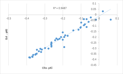
pKi= -1.1320 + 0.0237(±0.0015) S1k+ 0.0532(±0.0121) CATS3D_15_DL + 0.8302(±0.1317) MP -0.0158(± 0.0104) SHED_NL + 0.0325(±0.0148) VE3sign_B(s) (5) N= 47, R2= 0.9490, R2 Adj . = 0.9410, R2 cv= 0.947, F = 152.577, Q=1128.3991 S1K = 1-path kier alpha- modified shape index (topological indices) Mp = Mean atomic polarizability (scaled on carbon atom) (constitutional indices) AROM = Aromaticity index (geometrical descriptors) CATS3D_15_DL = CATS3D donor- lipophilic BIN 15 CATS3D_14_AP = CATS3D acceptor – positive BIN 14 The activity value pKi for the data set has been estimated using the best five-parametric model. The estimated values are in good agreement with the observed pKi values (Table 5) showing that five-parametric model is good for modeling the activity of present set of compounds. The predictive power of the model comes out to be 0.9487 (Figure 1).

S.No.	R2 CV	SSY	PRESS	PRESS/SSY
1	0.695	0.515	0.157	0.305
2	0.831	0.575	0.097	0.169
3	0.843	0.581	0.091	0.157
4	0.847	0.583	0.089	0.153
5	0.847	0.583	0.089	0.153
6	0.847	0.583	0.089	0.153
7	0.851	0.585	0.087	0.149
8	0.853	0.587	0.086	0.147
9	0.859	0.589	0.083	0.141
10	0.859	0.589	0.083	0.141
11	0.871	0.596	0.077	0.129
12	0.899	0.611	0.062	0.101
13	0.9	0.612	0.061	0.1
14	0.9	0.612	0.061	0.1
15	0.902	0.613	0.06	0.098
16	0.902	0.613	0.06	0.098
17	0.904	0.613	0.059	0.096
18	0.904	0.614	0.059	0.096
19	0.907	0.616	0.057	0.093
20	0.914	0.619	0.053	0.086
21	0.916	0.62	0.052	0.084
22	0.935	0.632	0.041	0.065
23	0.937	0.633	0.04	0.063
24	0.938	0.633	0.039	0.062
25	0.94	0.633	0.038	0.06
26	0.94	0.634	0.038	0.06
27	0.943	0.636	0.036	0.057
28	0.947	0.638	0.034	0.053

Table 7: Cross validated parameters for various models.

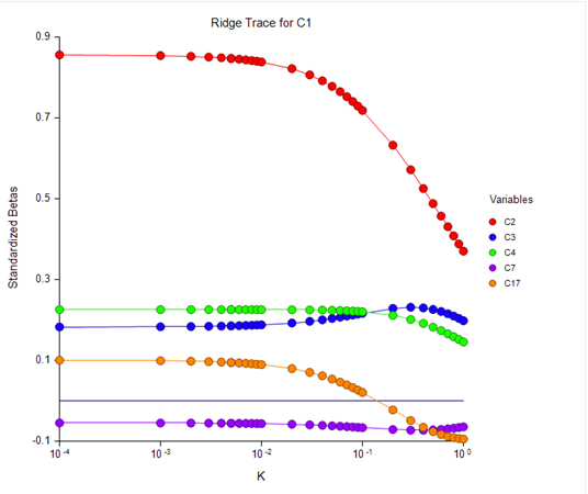
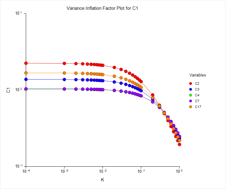
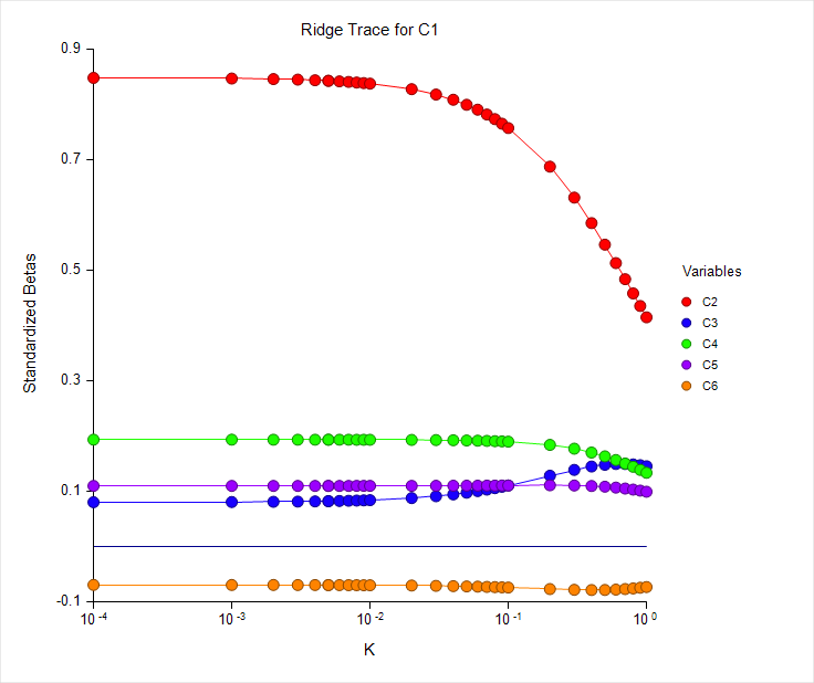
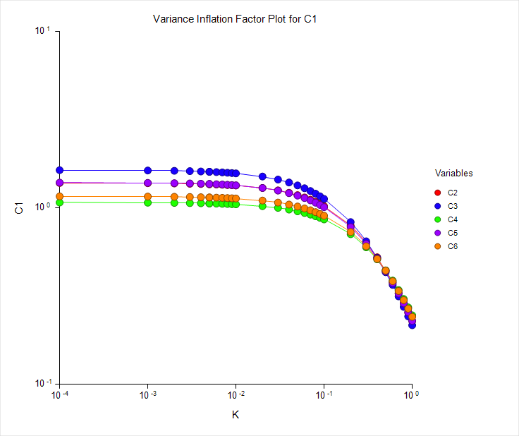
Figure 1: Graph between observed and estimated pKi values using best five-parametric model (Eq.5).

The results of Ridge analysis (Figure 2 & Table 6) also shows that the model is free from any kind of defect. The VIF (variance inflation factor) trace also confirms our finding. No collinearity has been observed in this model.

However, two compounds 6 and 42 have been found to be outliers. Therefore, they were deleted from the data. After deleting these two compounds, again regression analysis for four parametric and five-parametric models were carried out. The models obtained are reported below:

S.N0.	Observed pkI	Estimated pkI	Residual
1	-0.382	-0.382	0
2	-0.321	-0.33	0.009
3	-0.047	-0.023	-0.024
4	-0.07	-0.108	0.038
5	0.02	0.033	-0.013
6	0.064	-0.042	0.106
7	-0.018	-0.042	0.024
8	-0.099	-0.069	-0.03
9	-0.07	-0.038	-0.032
10	-0.102	-0.109	0.007
11	-0.084	-0.092	0.008
12	-0.084	-0.037	-0.047
13	-0.079	-0.083	0.004
14	-0.059	-0.061	0.002
15	-0.346	-0.346	0
16	-0.325	-0.302	-0.023
17	-0.334	-0.325	-0.009
18	-0.266	-0.26	-0.006
19	-0.317	-0.308	-0.009
20	-0.281	-0.301	0.02
21	-0.299	-0.296	-0.003
22	-0.264	-0.283	0.019
23	-0.264	-0.271	0.007
24	-0.264	-0.253	-0.011
25	-0.264	-0.245	-0.019
26	-0.143	-0.138	-0.005
27	-0.237	-0.21	-0.027
28	-0.219	-0.213	-0.006
29	-0.202	-0.222	0.02
30	-0.115	-0.131	0.016
31	-0.211	-0.197	-0.014
32	-0.193	-0.198	0.005
33	-0.175	-0.187	0.012
34	-0.188	-0.181	-0.007
35	-0.103	-0.113	0.01
36	-0.387	-0.379	-0.008
37	-0.369	-0.374	0.005
38	-0.37	-0.373	0.003
39	-0.352	-0.354	0.002
40	-0.365	-0.356	-0.009
41	-0.344	-0.312	-0.032
42	-0.194	-0.286	0.092
43	-0.229	-0.219	-0.01
44	-0.201	-0.156	-0.045
45	-0.244	-0.225	-0.019
46	-0.369	-0.373	0.004
47	-0.351	-0.351	0

Table 8: Estimated activity values using model (5).

Figure 2: Ridge trace for the best five-parametric model.

Four-Parametric Model

In earlier four-parametric correlation the R2 value was observed to be 0.9461 and R2Adj. was found to be 0.9410. But when two outliers were removed these value show drastic improvement, In the R2cv value which was earlier 0.943 the new value comes out to be 0.9855. Similar observation has also been reported for Q value which also shows significant jump. The model comes out to be:, pKi= -0.6383+0.0232(±0.0006) S1K+0.7077(±0.0706) Mp + 0.0787(±0.0112)CATS3D_14_AP-0.4208(±0.0949) AROM (6) N = 45, R2 = 0.9857, R2Adj.= 0.9843, R2cv = 0.9855 , F = 691.338, Q=4705.21

Five- Parametric Model

Similarly, the five-parametric model discussed above also gave better results when the two compounds were removed from the data set. The R2 value changes from 0.9490 to 0.9897. That is the case with R2CV value also which changes from 0.947 to 0.9896. F-ratio also shows a quantum jump in the value. Q value also supports that after deleting the outliers the new five–parametric model with 45 compounds is the best for estimating the pKi values of the compounds used in the present study. pKi=-0.7111+0.0225(±0.0005) S1K+0.0231(±0.0060)CATS3D+0.7001(±0.0609)Mp +0.0612(±0.0107) CATS3D_14_AP+-0.3346(±0.0847) AROM (7) N= 45, R2 = 0.9897, R2 Adj .= 0.9884, R2cv = 0.9896, F =748.859,Q=6377.11 Using the best five-parametric model the pKi values were estimated which are in excellent agreement to the observed values. Such values are reported in Table10 . The cross-validated parameters also show improved staticstical values to the parameters which again confirm our findings.

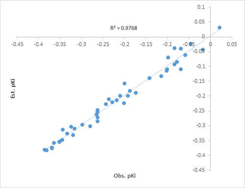
A graph has been ploted between observed and estimated pKi values using the best five-parametric model after deleting two outliers. Such graph is demonstrated in Fig. 4. The predictive power of the model comes out to be 0.98 which is much better than the five-parametric model obtained earlier with N=47.

The VIF parameters Table11 also suggest that the five-parametric model after deleting outliers is better. The model was tested using crossvalidated vparameters and also collinearity was tested using ridge analysis. The ridge plot obtained shows that all the parameters are acceptable and they are free from any type of defect including defect of collinearity.

Conclusions

On the basis of above discussion it is concluded that the antidiabetic activity in terms of pKi values can be modelled using 2d QSAR topological parameters. The obtained model is free from any kind of defect. More than 98% data is explained using this model. The Kier modified shape index has a negative coefficient showing that this parameter has a retarding effect towards pKi. Aromatic index AROM has also a negative coefficient meaning, thereby, that it has a negative role towards pKi activity value. All other parameters have positive coefficients revealing that they have positive effect on the activity depicted by pKi for the present set of compounds. The model tested using cross validation techniqu also supports the finding. The Q value for the proposed model is highest suggesting that model can be used for estinating and prdicting the pKi value of present set of compounds. The two compounds no. 6 and 42 are outliers. It appears they behaved differently. The reason may be the difference in the topology and behaviour of some of the attached groups which are strong electronegative in nature specially -Br. The compounds that are proposed in the light of present finding are supposed to serve as a good antidiabetic agents that can be used for theraputic purposes after some further in vivo investigations.

Model No.	Parameters Used	VIF	T	λ	K
22	S1K	2.25	0.45	1.89	1
	CATS3D	1.383	0.72	1	1.9
	Mp	1.032	0.97	0.98	1.9
	SHED_NL	1.039	0.96	0.85	2.2
	VE3sign_B(s)	1.68	0.6	0.27	6.9

Table 9: VIF Parameters for the best model (5).

Figure 3: VIF Plot for the best five-parametric model (Eq. 5).

Eq.	Parameters	A = (1….3) i	C	MSE	F-Ratio	R2	R2 Adj	Q=R/MSE
6	S1K	0.0232(±0.0006)	-0.6383	0.0002	691.34	0.9857	0.9843	4705.21
	Mp	0.7077(±0.0706)
	CATS3D_14_AP	0.0787(±0.0112)
	AROM	-0.4208(±0.0949)
	AROM	-0.4208(±0.0949)
7	S1K	0.0225(±0.0005)	-0.7111	0.0001	748.86	0.9897	0.9884	6377.11
	CATS3D	0.0231(±0.0060)
	Mp	0.7001(±0.0609)
	CATS3D_14_AP	0.0612(±0.0107)
	AROM	-0.3346(±0.0847)

Table 10: Quality of models after deleting compound no. 6 and 42.

Eq	R2 CV	SSY	PRESS	PRESS/SSY
6	0.9855	0.5835	0.0084	0.0145
7	0.9896	0.5859	0.0061	0.0104

Table 11: Cross validated parameters for the models after deleting two outliers.

Compd. N0.	Observed pKi values	Estimated pKi values	Residual
1	-0.382	-0.382	0
2	-0.321	-0.33	0.009
3	-0.047	-0.023	-0.024
4	-0.07	-0.108	0.038
5	0.02	0.033	-0.013
6	-0.018	-0.042	0.024
7	-0.099	-0.069	-0.03
8	-0.07	-0.038	-0.032
9	-0.102	-0.109	0.007
10	-0.084	-0.092	0.008
11	-0.084	-0.037	-0.047
12	-0.079	-0.083	0.004
13	-0.059	-0.061	0.002
14	-0.346	-0.346	0
15	-0.325	-0.302	-0.023
16	-0.334	-0.325	-0.009
17	-0.266	-0.26	-0.006
18	-0.317	-0.308	-0.009
19	-0.281	-0.301	0.02
20	-0.299	-0.296	-0.003
21	-0.264	-0.283	0.019
22	-0.264	-0.271	0.07
23	-0.264	-0.253	-0.011
24	-0.264	-0.245	-0.019
26	-0.143	-0.138	-0.005
26	-0.237	-0.21	-0.027
27	-0.219	-0.213	-0.006
28	-0.202	-0.222	0.02
29	-0.115	-0.131	0.016
30	-0.211	-0.197	-0.014
31	-0.193	-0.198	0.005
32	-0.175	-0.187	0.012
33	-0.188	-0.181	-0.007
34	-0.103	-0.113	0.01
35	-0.387	-0.379	-0.008
36	-0.369	-0.374	0.005
37	-0.37	-0.373	0.003
38	-0.352	-0.354	0.002
39	-0.365	-0.356	-0.009
40	-0.344	-0.312	-0.032
41	-0.229	-0.219	-0.01
42	-0.201	-0.156	-0.045
43	-0.244	-0.225	-0.019
44	-0.369	-0.373	-0.004
45	-0.351	-0.351	0

Table 12: Estimated pKi values from the best model after deleting two compounds.

Model No.	Parameters Used	VIF	T	λ	K
(Eq. 7)
7	S1K	1.3843	0.7224	1.912	1
	CATS3D	1.636	0.6112	1.0997	1.74
	MP	1.0723	0.9326	1.0283	1.86
	CATS3D_14_AP	1.3911	0.7189	0.543	3.52
	AROM	1.1621	0.8605	0.4167	4.59

Table 13: VIF Values after for the best five-parametric model deleting two outliers.

Figure 4: The predictive power of the model comes out to be 0.98 which is much better than the five-parametric model obtained earlier with N=47.

Figure 5: Ridge trace for the best five-parametric model (Eq. 7) after deleting two outliers.

Figure 6: VIF trace for the best five-parametric model Eq. 7 after deleting two utliers.

References

Wolff JL, Starfield B, Anderson G (2002) Prevalence, expenditures, and complications of multiple chronic conditions in the elderly. Arch Internal Medicine 162(20): 2269-2276.
Venkat Narayan KM, Boyle PJ, Geiss LS, Saaddine JB, Thompson TJ (2006) Impact of recent increase in incidence on future diabetes burden US, 2005-2050. Diabetes Care 29(9): 2114-2116.
Anderson AR (2000) Chromium in the prevention and control of diabetes. Diabetes Metabolism 26(1): 22-27.
Cefalu WT, Hu FB (2004) Role of chromium in human health and in diabetes. Diabetic Care 27(11): 2741-2751.
Vaibhav AD, Prasad VB (2013) SAR and computer aided drug design approaches in the discovery of peroxisome proliferator activated receptor 𝛾 activators: a perspective. Journal of Computational Medicine.
Tripathi RB, Jain J, Siddiqui AW (2018) Design of new peroxisome proliferators gamma activated receptor agonists (PPARγ) via QSAR based modeling. Journal of Applied Pharmaceutical Science and Research 1 (1): 23- 26.
Pantaleao SR, Fujii DGV, Maltarollo VG, Silva DC, Trossini GHG, et al. (2017) The role of QSAR and virtual screening studies in Type 2 diabetes drug discovery. Medicinal Chemistry 13(8): 706-720.
Chawla AM, Chawla PY, Dhawan RK (2014) QSAR study of 2,4-dioxothiazolidine antidiabetic compounds. Der Pharmacia Chemica 6(2): 103-110.
Kesar S, Mishra P, Ojha P, Singh S (2016) 2D QSAR study of potent GSK3β inhibitor for treatment of type II diabetes. International Journal of Pharmaceutical Science and Research 7: 2932-2943.
Zivkovic JV, Trutic NV, Veselinovic JB, Nikolic GM, Veselinovic AM (2015) Monte Carlo method based QSAR modelling of maleimide derivatives as glycogensynthasekinase-3β inhibitors. Computers in Biology and Medicine 64: 276-282.
Vyas VK, Bhatt HG, Patel PK, Jalu J, Chintha C, et al. (2013) CoMFA and CoMSIA studies on C-aryl glucoside SGLT2 inhibitors as potential antidiabetic agents. SAR and QSAR in Environmental Research 24(7): 519- 551.
Lorca M, Morales-Verdejo C, VásquezVelásquez D, Andrades-Lagos J, CampaniniSalinas J, et al. (2018) Structure activity relationships based on 3DQSAR CoMFA/CoMSIA and design of aryloxypropanol-amine agonists with selectivity for the human β3-adrenergic receptor and anti-obesity and antidiabetic profiles. Molecules 23(5): 1191.
Manoj KM, Rajnish K, Priyanka M (2014) In silico accounting of novel pyridazine analogues as h-PTP 1B inhibitors: pharmacophoremodelling, atombased 3D QSAR and docking studies. Medicinal Chemistry Research 23: 2701-2711.
Saxena A, Agrawal VK, Khadikar PV (2003) Estimation of antitumor activity of sulphonimidamide analogous of oncolytic sulphonylureas. Oxidation Communication. 26: 9-13.
Agrawal VK, Sharma R, Khadikar PV (2002) QSAR Studies on Carbonic Anhydrase Inhibitors:A Case of Ureido and Thioureido Derivatives of Aromatic/Heterocyclic Sulfonamides. Bioorganic Medicinal Chemistry 10(9): 2993-2999.
Agrawal KV, Khadikar PV (2003) Modeling of Carbonic Anhydrase Inhibitory Activity of Sulfonamides Using Molecular Negentropy. Bioorganic Medicinal Chemistry Letters 13(3): 447-453.
Agrawal VK, Shrivastava S, Khadikar PV Supuran CT (2003) Quantitative Structure-Activity Relationship Studies on Sulfanilamide Schiff Bases: CAInhibitors Bioorganic Medicinal Chemistry. 11: 5353-5362.
Agrawal VK, Bano S, Supuran CT, Khadikar VP (2004) QSAR study on carbonic anhydrase inhibitors: aromatic/heterocyclic sulfonamides containing 8-quinoline- sulfonyl moieties, with topical activity as antiglaucomaagents. European Journal of Medicinal Chemistry 39(7): 593-600.
Agrawal VK, Singh J, Banerji M, Gupta M, Khadikar PV, et al. (2005) QSAR Study On Carbonic Anhydrase Inhibitors: Water-Soluble Sulfonamides Incorporating -Alanyl Moieties, Possessing Long Lasting-Intra Ocular Pressure Lowering Properties -A Molecular Connectivity Approach. European Journal of Medicinal Chemistry 40(10): 1002-1012.
Khadikar PV, Clare BW, Balaban AT, Supuran CT, Agarwal VK, et, al. (2006) QSAR of CAI, CAII, and CA IV Inhibitory Activities: Relative Correlation Potential of Six Topological Indices. Roum 5: 703-717.
Khadikar PV, Deeb O, Jaber A, Singh J, Agrawal VK, et al. (2006) Development of Quantitative structure activity relationship for a set of Carbonic anhydrase inhibitors: Use of Quantum and Chemical Descriptors. Letters in Drug Design & Discovery 3(9): 622-635.
Singh J, Lakhwani M, Khadikar PV, Agrawal VK, Supuran CT, et al. (2006) QSAR Study on Murine Recombinant Isozyme mCAXIII: Topological Vs Structural Descriptors. Arkivoc 2006(14): 103-118.
Singh J, Shaik B, Singh S, Sikhima S, Agrawal VK, et al. (2007) QSAR studies on the activation of the human carbonic anhydrase cytosolic isoforms I and II and secretory isozyme VI with amino acids and amines. Bioorganic & Medicinal Chemistry 15(20): 6501-6509.
Singh J, Shaik B, Singh S, Agrawal VK, Khadikar PV, et al. (2008) Comparative QSAR Study on Para-substituted Aromatic Sulphonamides as CAII Inhibitors: Information vs Topological (distance-based and connectivity) Indices. Chemical Biology Drug Design 71(3): 244-259.
Chang LL, Sidler KL, Cascieri MA, Laszlo SD, Koch G, et al. (2001) Substituted imidazoles as glucagon receptor antagonists. Bioorganic and Medicinal Chemistry Letters 11(18): 2549-2553.
Borras J, Scozzafava A, Menabuoni L, Mincione F, Briganti F, et al. (1999) Carbonic anhydrase inhibitors: synthesis of watersoluble, topically effective intraocular pressure lowering aromatic/heterocyclic sulfonamides containing 8-quinoline-sulfonyl moieties: is the tail more important than the ring?. Bioorganic and Medicinal Chemistry 7(11): 2397-2406.
Vullo D, Franchi M, Gallori E, Antel J, Scozzafava A, et al. (2004) Carbonic anhydrase inhibitors. Inhibition of mitochondrial isozyme V with aromatic and heterocyclic sulfonamides. Journal of Medicinal Chemistry 47(5): 1272-1279.
Winum JY, Dogne JM, Casini A, De Leval X, Montero JL, et al. (2005) Carbonic anhydrase inhibitors: Synthesis and inhibition of cytosolic membrane-associated carbonic anhydrase isozymes I, II, and IX with sulfonamides incorporating hydrazino moieties. Journal of Medicinal Chemistry 48(6): 2121-2125.
Ravichandran V, Harish R (2019) QSAR studies on imidazoles and sulfonamides as antidiabetic agents. Ovidius University Annals of Chemistry 30(1): 5-13.

← Previous Article A Systematic Review on Concentration of Heavy Metal in the Ambient Air of Different Industries and the Health Risk Assessment Next Article → Do Genes Play a Role in Allergic Rhinitis?

QSAR Studies on Some Sulfonamides as Antidiabetic Agents

Introduction

Presentation of Data

Results and Discussion

One- Parametric Model

Two-Parametric Model

Three-Parametric Model

Four-Parametric Model

Five-Parametric Model

Four-Parametric Model

Five- Parametric Model

Conclusions

References

Cite this article