Implementation of a Real-Time, Data-Driven Online Epidemic Calculator for Tracking the Spread of COVID-19 in Singapore and Other Countries
While there are many online data dashboards on COVID-19, there are few analytics available to the general public to help them gain a deeper insight into the COVID-19 pandemic and evaluate the effectiveness of social intervention measures. To address the issue, this study describes the methods underlying the development of an online COVID-19 Epidemic Calculator for tracking COVID-19 growth parameters. From publicly available infection case and death data, the calculator is used to estimate the effective reproduction number, doubling time, final epidemic size, and death toll. As a case study, we analyzed the results for Singapore during the “Circuit breaker” period from April 7, 2020 to the end of May 2020. The calculator shows that the stringent measures imposed have an immediate effect of rapidly slowing down the spread of the coronavirus. After about two weeks, the effective reproduction number reduced to about 1.0. Since then, the number has been fluctuating around 1.0 for more than a month. The COVID-19 Epidemic Calculator is available in the form of an online Google Sheet and the results are presented as Tableau Public dashboards at www.cv19.one. By making the calculator readily accessible online, the public can have a tool to meaningfully assess the effectiveness of measures to control the pandemic.
Fook Fah Yap1* and Minglee Yong2
Introduction
As countries around the world take drastic measures to contain the COVID-19 pandemic, people need to understand the effectiveness of such interventions. Making sense of epidemiological data can be challenging given confusing and overlapping terminology. Raw data and statistics on infection numbers (Figure 1) do not directly help answer the following questions:
- Are social distancing measures working?
- How much longer does it take to flatten the curve?
- What will be the final death toll?
This paper describes the methods underlying an online COVID-19 Epidemic Calculator for tracking and estimating COVID-19 growth parameters, including reproduction number, doubling time, final epidemic size, and death toll. These methods are illustrated using the case example of Singapore. We demonstrate how the calculator can reveal the effect of imposing strict social distancing measures (“Circuit breaker”) from April 7, 2020 that is not apparent from just looking at infection numbers.
While our methodology is similar in certain aspects to several freely available software packages and programming codes for calculating the effective reproduction number [2, 3, 4, 5], we differ from those work because we implement real-time, data-driven calculations in the widely used Excel spreadsheet, with sub-minute execution time, even for calculating a 4-month, 100-country data set. Furthermore, this calculator is readily available as an online Google Sheet to facilitate sharing and collaboration. The input data for the calculator is obtained from publicly available sources [6, 7, 8] and is automatically updated daily.
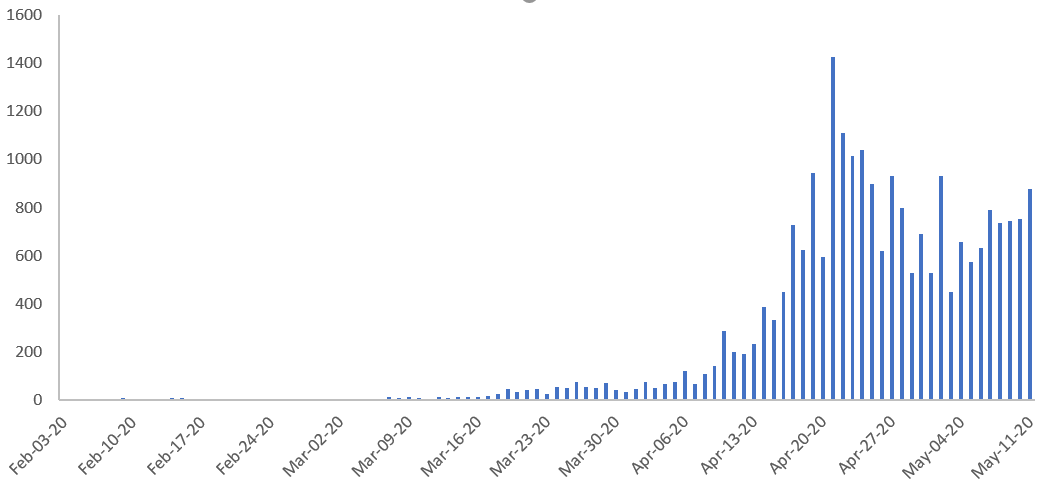
![Figure 1: Total Confirmed Cases in Singapore [1].](/fulltextimages/6651/fig_1.png)
Introduction to Terminology
Figure 2 identifies the different overlapping terms used in epidemiology and illustrates the timeline for the various stages of infection. These terms and variables will be used for calculating parameters that can help us understand and monitor the spread of the COVID-19 infection in a country.
Exposed is the state at which an individual first becomes infected but is not yet contagious. The latent period is the time from being infected (exposed) to becoming contagious. An infected person can be contagious even before the onset of symptoms. Data suggests that some people could have infected others 1 to 3 days before they developed symptoms [9, 10].
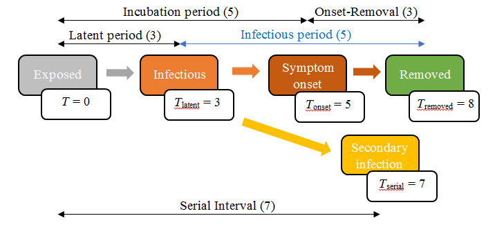
The incubation period is the time from exposed to the onset of symptoms. The mean incubation period for COVID-19 is estimated to be 5 days [11, 12]. The infectious period is the time between becoming contagious to the time of removal or recovery. Hence, it is the difference between the time of removal and the latent period (Tremoved–Tlatent).
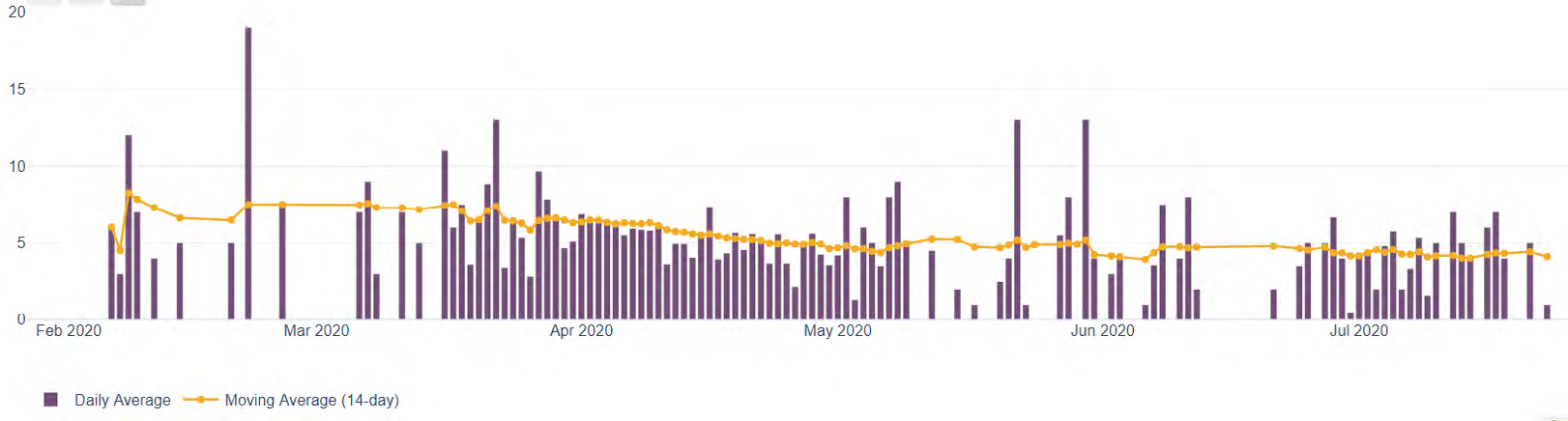
In Singapore, the 14-day average time from the onset of symptoms to removal ranges from 1.5 to 6 days after the start of the Circuit breaker on April 7, 2020 (Figure 3). The serial interval is the time when a secondary infection is generated. For COVID-19 in Singapore, the serial interval between transmission pairs ranges between 3 days and 8 days [13].
Other researchers have reported serial intervals within the same range [12, 14, 15, 16].
Critical Parameters
The rate of infection growth in a population can be estimated using the effective reproduction number. The effective reproduction number is the number of secondary cases directly being infected by a primary case in a population. Social distancing measures should reduce the spread of infection and this would be reflected by a reduction in the effective reproduction number. Hence, monitoring the effective reproduction number over time will allow us to evaluate if social distancing measures or any other interventions are working. We will demonstrate how to estimate the effective reproduction number using a non- parametric approach, as well as a Bayesian approach. We will also show how to derive estimates of dates of actual symptom onset and dates of being exposed which are important for our estimation of the effective reproduction number.
Another parameter that can be used to estimate the rate of infection growth is the doubling time. This is the time for the total number of cases to double in a population, given the current infection rate. Hence, effective interventions to curb the spread of an infection should increase the doubling time. We will estimate the doubling time by assuming an exponential growth model [17]. Estimating the time needed to flatten an epidemic curve is an important part of forecasting the scope of an infectious disease outbreak. When new cases are significantly reduced, social distancing restrictions can be relaxed and other less intrusive measures can be put in place. In this study, we will show how logistic and Gompertz models can be used for forecasting the future number of cases and deaths over time using only publicly available data. These numbers will allow us to gauge the vulnerability of the population and quantify the direct health impact of COVID-19.
Since these parameters are useful to help the general public understand about the spread of COVID-19 in their countries, as well as in other countries and regions, the objective of this research study is to develop a readily available online COVID-19 Epidemic Calculator to provide estimates of the critical parameters described here. The interested public can access this online calculator to gain a deeper insight into the COVID-19 pandemic, as well as to evaluate the effectiveness of a range of public health and social intervention measures [18].
Methodology
Method for Calculating the Effective Reproduction Number for Estimating How Fast COVID-19 is Spreading in a Country
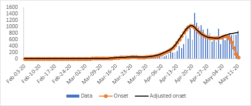
Step 1: Deriving symptom onset dates from confirmation dates The daily number of reported cases is partly dependent on the number of tests conducted, which may be variable due to factors such as testing capacity and the day of week. To account for this variation, we perform a running 7-day average of test cases. Other methods of applying a smoothing filter to the time series may be used if appropriate.
Another issue is the delay between the onset of symptoms and case confirmation (removal or isolation). Case onset dates can be derived if records of onset-to- confirmation dates are available for every individual (Figure 3). Otherwise, case onset dates can be estimated by using the following procedure.
- For each date, distribute case counts back in time according to a Poisson distribution with a mean of 3 days (symptom onset to removal) as illustrated in Figure 4.
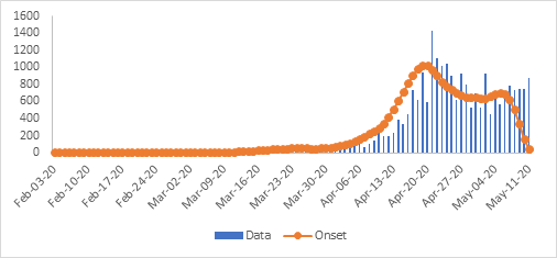
- Sum the back distributed case counts for each date to derive the onset curve as shown in Figure 5.
Distributing reported cases back in time and recreating the onset curve result in a “right-censored” time series. This means that there are onset cases close to the present date that are yet to be reported. We correct this by estimating the percentage of onset cases on Day (t-a) that have not yet been reported by today (Day t). We can use the cumulative distribution function of the Poisson “onset-to-removed” distribution to adjust for the number of onset cases, thus removing right censoring [19].
Adjusted onset:
Adjusted onset =
(
from present date)
$$ \frac {O n s e t}{P (D e l a y \leq D a y s \mathrm {f r o m}} $$
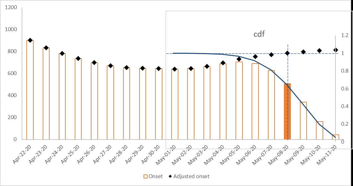
Consider an example illustrated in Figure 6. Three days ago, there were 470 reported onset cases. This represents the fraction of the actual number reported over the next 3 days. This fraction is equal to the value of the cumulative distribution function of our Poisson distribution at Day 3, which is 65%. Hence, the current count of onset on that day represents 65% of the actual total. After adjustment, the actual total is estimated to be (1/0.65) of 470, which is 723. Figure 7 shows the adjusted onset curve.
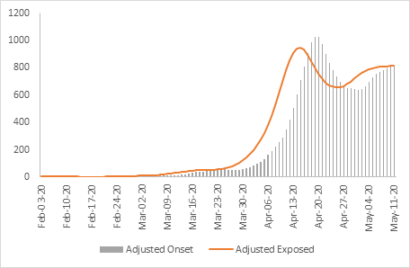
Step 2: Deriving infection (exposed) dates from onset dates A similar procedure as in Step 1 can be applied to the onset counts to derive the infection (exposed) time series.
Figure 8 shows the adjusted exposed time series where the incubation period (from exposed to symptom onset) follows a Poisson distribution with a mean of 5 days.
Step 3: Estimating the Effective Reproduction Number, R(t) The basic reproduction number, R_0_, is the expected number of infections directly generated by one case given that all individuals are equally susceptible. As the infection spreads, the susceptibility of the population decreases. The effective reproduction number, R_(t), is related to the basic reproduction number, R0, by R(t)=R0S(t), where S(t) is the average susceptibility of the population. R(t) is often used as an indicator of the effectiveness of interventions, such as social distancing measures, to contain the spread of a virus. If R(t) is greater than 1.0, the infection is growing at an exponential rate. If R(t) is at 1.0, the spread is sustained at a linear rate. If R(t) is less than 1.0, the infection is spreading at a slower pace and will eventually die out. Although R(t)_ cannot be measured directly, it can be estimated in different ways. We describe two methods that can be implemented in a spreadsheet without any programming codes.
Bayesian Approach: The Bayesian approach allows us to continuously update our estimate of a set of parameters, Θ, as more data becomes available.
$$ P (\Theta \mid \mathrm {d a t a}) = \frac {P (d a t a \mid \Theta) . P (\Theta)}{P (d a t a)} $$ P(Θ), the prior distribution, represents our prior estimates about the true value of Θ. P(data|Θ) is the likelihood distribution. It is also often written as L(Θ|data) which means the probability of observing the data given Θ. For the method to work, it is necessary to calculate the likelihood distribution for all possible values of Θ. P(data) is the model evidence and it is the same for all possible hypotheses (values of Θ) being considered. P(Θ│data_)_ is the posterior distribution and represents our updated estimate of the value of Θ given the observed data [20].
The main objective of Bayesian inference is to calculate the posterior distribution of our parameters using our prior beliefs updated with our likelihood. From the posterior distribution, we can determine the most likely values of Θ given the observed data. Since we are usually only interested in relative probabilities of different hypotheses, P(data) can be left out of the calculation and we write the model form of Bayes’ theorem as ( | data) ( | ). ( ) P P data P Θ ∝ Θ Θ (1) Where ∝ means “proportional to”. For estimating R_t_, the Bayes’ theorem that we use is ( \ k ) ( \ ). ( ) t t t t t P R P k R P R ∝ (2) Where the data, kt, is the daily number of cases, and the parameter, Rt, is the effective reproduction number. Equation (4) is updated every day by using yesterday’s posterior, P(R(t-1)│k(t-1)), to be today’s prior P(Rt). On day two, the equation becomes
2 2 2 2 1 1 1 ( \ k ) ( \ ). ( \ ). ( ) P R P k R P k R P R ∝ (3) So generally, T $$ \propto P \left(R _ {1}\right). \prod_ {t = 1} ^ {T} P \left(\mathrm {k} _ {t} \mid R _ {t}\right) \tag {4} $$
1 1 ( | k ) ( ). (k | )
T T t t t P R P R P R
Assuming a uniform starting prior P(R1), this reduces to:
T $$ ) \propto \prod_ {t = 1} ^ {T} P \left(\mathrm {k} _ {t} \mid R _ {t}\right) \tag {5} $$
1 ( | k ) (k | )
T T t t t P R P R
Note that the posterior on any given day is equally influenced by the distant past as much as the recent day. This is fine if we are estimating a static parameter that does not change with time. However, the value of Rt is dynamic and is more closely related to recent values than older ones. To address this issue, we can adopt Systrom’s approach [2] of only incorporating the last m days of the likelihood function:
T $$ ) \propto \prod_ {t = 1 - m} ^ {T} P \left(\mathrm {k} _ {t} \mid R _ {t}\right) \tag {6} $$
1 ( | k ) (k | )
T T t t t m P R P R
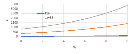
Bettencourt & Ribeiro’s Likelihood Function: To calculate the likelihood function L(Rt│kt)=P(kt│Rt), we first assume that the number of new infections on any given day can be described by a Poisson probability distribution with a mean of λ. The probability of seeing k new cases is ke P k k λ λ λ $$ \propto \frac {\lambda^ {k} e ^ {- \lambda}}{k !} (7) $$ ( | ) !
Bettencourt & Ribeiro [21] has derived an equation relating Rt to λ.
$$ \lambda = k _ {t - 1} e ^ {\gamma \left(\mathrm {R} _ {t} - 1\right)} \tag {8} $$ Where γ is the reciprocal of the serial interval (see Figure 2). Figure 9 shows the variation of λ with Rt for some values of kt-1.
Equations (9) and (10) allow us to reformulate the likelihood function as a Poisson distribution, parameterized by fixing k and varying Rt.
k $$ = P \left(k \mid R _ {t}\right) = \frac {\lambda^ {k} e ^ {- \lambda}}{k !} \tag {9} $$ t t e L R k P k R k ( | ) ( | ) !
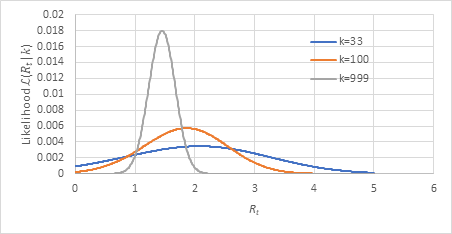
Figure 10 shows that as k increases, the peak value of the likelihood function L(Rt|k) increases and the distribution becomes less spread out about. This means that as the number of infections increases the confidence of our Rt estimate should improve.
In evaluating the posteriors, it is more convenient to use the logarithm of the likelihood function.
$$ \ln \left(L \left(R _ {t} \mid k\right)\right) = k \left[ \ln \left(k _ {t - 1}\right) + \lambda \left(\mathrm {R} _ {t} - 1\right) \right] - \mathrm {k} _ {t - 1} e ^ {\gamma \left(R _ {t} - 1\right)} - \ln (k!) \tag {10} $$ To perform the Bayesian update, we can do a sum of the log- likelihoods over the last m days and then exponentiate to get the likelihood. From equations (8) and (12), = + = + − − + ∑ ∑ ( 1) 1 1 ln( ( | )) ln( ( | )) constant k [ln( ) (R 1)] k e constant t T T R t T t t t t t t t T m t T m P R k L R k k γ γ − − − = − = − (11) From the posterior distribution (Figure 11) we can also obtain the confidence interval for Rt.
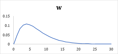
Non-Parametric Approach: Wallinga J, et al. [22, 23] have developed a non-parametric method to derive the reproduction number from the exponential growth rate, ( ) ( ) ( ) ( ) o $$ R (t) = \frac {c (t)}{\int_ {0} ^ {\infty} c (t - a) w (a) d a} $$ (12) Where c(t) is the rate of new infections at time t, and w(a) is the probability density function of the serial interval (Figure 2).
The serial interval is the time from being infected to generating a secondary infection. We assume a gamma distribution with a mean serial interval of 7 days and a peak (most infectious) at Day 4 (Figure 12). This accounts for a latent period where the exposed individual is not yet infectious. Equation (14) can be evaluated in a spreadsheet using the infection data derived above and a numerical integration scheme.
Method for Calculating the Doubling Time for Estimating How Fast COVID-19 is Spreading in a Country
Another parameter often used to measure infection rate in a population is the doubling time, defined as the time for cumulative cases to double based on the current growth rate [24].
( ) rt C t C e $$ \begin{array}{l} C (t) = C _ {0} e ^ {r t} \\ C \left(t + T _ {d}\right) = C _ {0} e ^ {r \left(t + T _ {d}\right)} = 2 C _ {0} e ^ {r t} \\ \end{array} $$
0 (13) ( ) 0 0
r t T rt d
( ) 2 d $$ \left(t + T _ {d}\right) = C _ {0} e ^ {r \left(t + T _ {d}\right)} = 2 $$ Where C0 is the initial number of cases, Td is the doubling time, and r is the exponential growth rate. Taking the logarithm on both sides of the equation, ln( ( )) ln( ) C t C rt = +
0 (14) ln( ( )) ln( ) ( ) ln(2) ln( )
C t T C r t T C rt
$$ \left(t + T _ {d}\right)) = \ln \left(C _ {0}\right) + r \left(t + T _ {d}\right) = \ln (2) + \ln \left(C _ {0}\right) + r $$
0 0 d d ln(2) T r
= d As the growth rate slows, the doubling time increases accordingly. Note that the gradient of the ln(C(t)) curve is equal to r. Time-varying estimates of the doubling time can be made with a 7-day sliding window by iteratively fitting a linear regression model to ln(C(t)).
Method for Forecasting the Final Total Number of Cases and Deaths
When the growth rate is slowing down (Rt<1), we can project the final total cases and death counts by fitting publicly available data to a logistic model. The logistic model is often used to describe the shape of the cumulative epidemic curve (Figure 13) where the number of infected cases grow exponentially at first, then slows down, and finally flattens to a maximum limit. The final epidemic size can be estimated based on this slowing growth.
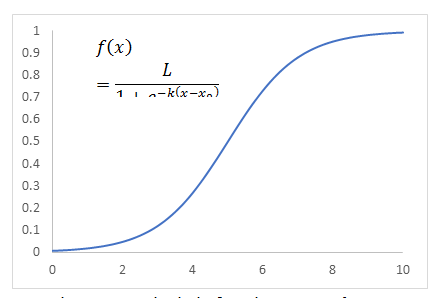
For our application, the total number of cases at time t can be approximated by Ma J [25]
C C C t
( ) $$ ) = \frac {C _ {F} C _ {0}}{C _ {0} + \left(C _ {F} - C _ {0}\right) e ^ {- \frac {r C _ {F}}{C _ {F} - C _ {0}} - t}} $$
0 F rC t C C F
(15) F ( ) C C C e + −
0 F
0 0 Where r is the exponential growth rate, C0 and CF are the initial and final numbers, respectively.
To find the best curve fit to the data and an estimate for CF, we use the maximum likelihood method. We assume that the number of reported cases, xi, at time, ti, follows the Poisson distribution and has a mean of μi, where μi is the calculated number of cases at time, ti.
$$ = x _ {i}) = \frac {\mu_ {i} ^ {x} e ^ {- \mu_ {i}}}{x !} \tag {16} $$
i x i i i i
e P x x (X ) !
Then, the log-likelihood function to be maximized is
1 n − $$ \sum_ {i = 0} ^ {n - 1} - \mu_ {i} + x _ {i} \ln \mu_ {i} (1 7) $$
0 ln i i i i x µ µ We choose the parameter values for CF and r that maximize the log-likelihood function. This can be done by using the Solver function in Excel. The parameter CF is estimated over a rolling window of, say 60 days, to obtain a moving update. See Figure 14.
Some research [26, 27, 28, 29] have also suggested that another
parametric model that can be used for forecasting COVID-19 case or death count is the Gompertz function, defined as t e $$ = C _ {F} \left(\frac {C _ {0}}{C _ {F}}\right) ^ {e ^ {- \gamma t}} $$ C C t C C
0 ( ) (18) F F
It is a special case of the generalized logistic function. The final value asymptote of the function is approached more slowly by the curve than the initial value asymptote, unlike the simple logistic function in which both asymptotes are approached by the curve symmetrically. For example, Figure 14 shows the cumulative death overtime for a few countries that clearly illustrate the asymmetry.
![Figure 14: Some research [26-29] have also suggested that another](/fulltextimages/6651/fig_14.png)
Results and Discussion
Evaluating the Effectiveness of Social Distancing Measures using Effective Reproduction Number
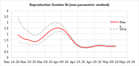
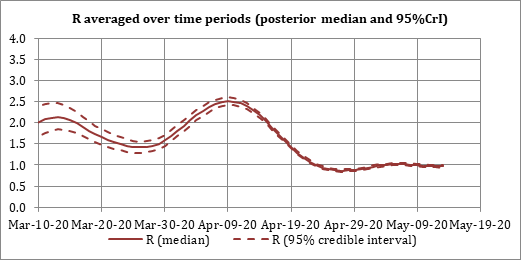
Figures 15 and 16 show the most likely values of Rt and the confidence interval over time for Singapore during the Circuit breaker period calculated using the Bayesian approach and non-parametric approach, respectively. The serial interval is assumed to be a Gamma distribution with a mean of 7 days and a mode of 4 days (standard deviation = 4.6 days). We can see that Rt changes with time and the confidence interval narrows with more data. The results are generally in good agreement with those calculated using the EpiEstim code (Figure 17) [3, 4].
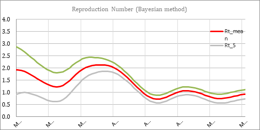
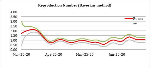
The results clearly show that the Circuit breaker measures imposed from April 7, 2020 have an immediate effect of rapidly slowing down the spread of COVID-19. We can also see that Rt settled to around 1.0 after about two weeks. Since then, the infection rate has remained sustained for more than a month. Given that dormitory residents make up the majority of the infected individuals, it can be concluded that individuals continue to infect others with a reproductive ratio of approximately 1 to 1 in that setting during the Circuit Breaker period as depicted in Figure 18 [30].
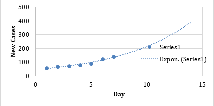
One problem with the calculation method is that it can only provide a good estimate for the reproduction number up to about one to two weeks before the current date. This is due to the time lag between infection and confirmation. As we get closer to the present day, the calculated mean value of Rt always tends to 1. For example, suppose that today is April 10, 2020, and case data is only available up to this date. Figure 19a shows that the calculated Rt values after April 3 do not reflect the true values as shown in Figure 18.
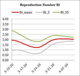
Figure 19a: Rt. tends to 1 as it approaches the current date.
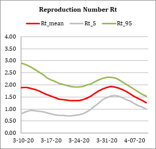
Figure 19b: Rt. adjusted by extrapolating next week’s cases from this week’s data.
Since the calculation cannot provide reliable estimates for current Rt based on real time data, it somewhat limits the usefulness of the metric for tracking infection spread. To alleviate this limitation, we do an exponential regression on the latest week’s case data and project the trend forward by one week (Figure 20). The results, shown in Figure 19b, give a much better estimate for the current values of Rt.
Evaluating the Effectiveness of Social Distancing Measures using Doubling Time
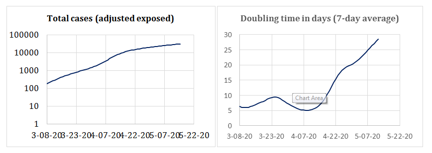
Figure 21 shows the log plot of the accumulated cases and the doubling time calculated using the method described in 2.2. Again, we can directly see the positive effect of the Circuit breaker measures that started on April 7, 2020. From a low point of about 5 days the doubling time has increased to about 4 weeks in slightly more than a month (Figure 22) [31, 32].
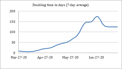
Although both the effective reproduction number and doubling time are directly related to the rate of infection growth, they provide us with different perspectives. The doubling time index has a time dimension. On the other hand, the effective reproduction number gives us a sense of the risk of an epidemic and whether interventions have brought it under control. Rt is useful in assessing in real time whether an infectious disease will persist.
How Much Longer Does It Take To Flatten The Curve? Forecasting Final Case and Death Counts.
Figure 23 shows the projected cases for Singapore calculated according to the method described in 2.3 and using a two- month data set.
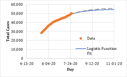
Table 1 shows the forecasts for a few countries including Singapore and how they compare with the projections by the Institute for Health Metrics and Evaluation (IHME) [33] at University of Washington Medicine. The projections by the IHME are based on more complex analytics and take into account factors such as changes in social distancing measures, diagnostic capability, and hospital capacity. Given that we did not directly account for these factors, our forecasts of the total number of cases and deaths may be considered indicative only. Assuming current prevailing conditions in the populations, results from the COVID-19 Epidemic Calculator are likely to be realistic estimates.
| Country | D , initial death count on May 0 20 2020 | Total death for Nov 1 2020 by Gompertz function fit | IHME projection for Nov 1 2020 |
|---|---|---|---|
| Singapore | 22 | 28 | 27 |
| USA | 97,222 | 186,285 | 219864 (141,969-284,123) |
| UK | 35,704 | 47,105 | 51274 (48,025-60,078) |
| Brazil | 18,894 | 134,781 | 177235 (81,623-191,443) |
Table 1: A comparison of the projected total deaths from the COVID-19 calculator as at July 25 2020, using data from the last two
Conclusion
show that the Circuit breaker measures imposed from April 7, 2020 in Singapore had an immediate effect of rapidly slowing down the spread of the COVID-19. Additionally, the results also reveal that the effective reproduction number has settled to around 1.0 after about two weeks. Since then, it has remained at that level for more than a month. This indicates that the infection rate among the dormitory residents is sustained and not likely to be reduced until this group become less susceptible.
This paper describes the methods underlying the online COVID-19 Epidemic Calculator for tracking COVID-19 growth parameters. From publicly available data, the calculator is used to estimate the distributions at time of symptom-onset and infection, effective reproduction number, doubling time, final epidemic size, and death toll for Singapore and other countries. The calculator and the associated graphs clearly
The COVID-19 Epidemic Calculator is available in the form of an online Google Sheet [34, 35] that imports daily infection data from the European Centre for Disease Prevention and Control [8]. The results are presented online as dashboards on Tableau Public (Figure 24) [36, 37]. It has the advantage of fast execution time without the need for any specialized software package or programming script. Users can also interact with the models by changing the parameters. Comparing with other similar work, our parameter estimates are found to be in good agreement with those estimated using different models and software. By making the COVID-19 Epidemic Calculator readily accessible online, it is hoped that the public and interested learners have the tool to meaningfully assess our effort in fighting COVID-19.
References
-
COVID-19 Situation Report, Ministry of Health Singapore.
-
Systrom K (2020) The Metric We Need to Manage COVID-19. Rt: the effective reproduction number.
-
Cori A, Ferguson NM, Fraser C, Cauchemez S (2013) A new framework and software to estimate time-varying reproduction numbers during epidemics. Am J Epidemiol 178(9): 1505-1512.
-
Abbott S, Hellewell J, Thompson RN, Sherratt K, Gibbs HP (2020) Temporal variation in transmission during the COVID-19 outbreak. Epiforecasts.
-
Boelle PY, Obadia T (2015) R0: estimation of R0 and real- time reproduction number from epidemics.
-
Coronavirus Source Data. Our World in Data.
-
The COVID Tracking Project.
-
Data on the geographic distribution of COVID-19 cases worldwide.
-
(2020) Report of the WHO-China Joint Mission on Coronavirus Disease 2019 (COVID-19). World Health Organization.
-
We WE, Li Z, Chiew CJ, Yong SE, Toh MP, et al. (2020) Presymptomatic Transmission of SARS-CoV-2-Singapore, January 23-March 16. MMWR 69(14): 411-415.
-
Lauer SA, Grantz KH, Bi Q, Jones FK, Zheng Q, et al. (2020) The incubation period of coronavirus disease 2019 (COVID-19) from publicly reported confirmed cases: estimation and application. Ann Intern Med 172(9): 577-582.
-
Bi Q, Wu Y, Mei S, Ye C, Zou X, et al. (2020) Epidemiology and transmission of COVID-19 in 391 cases and 1286 of their close contacts in Shenzhen, China: a retrospective cohort study. The Lancet Infectious Diseases 20(8): 911- 919.
-
Rachael P, Chiew CJ, Young BE, Chin S, Chen MIC, et al. (2020) Investigation of three clusters of COVID-19 in Singapore: implications for surveillance and response measures. Lancet 395(10229): 1039-1046.
-
Qun L, Guan X, Wu P, Wang X, Zhou L, et al. (2020) Early transmission dynamics in Wuhan, China, of novel coronavirus–infected pneumonia. N Engl J Med 382: 1199-1207.
-
Hiroshi N, Linton NM, Akhmetzhanov AR (2020) Serial interval of novel coronavirus (COVID-19) infections. Int J Infect Dis 93: 284-286.
-
Du Z, Ku X, Wu Y, Wang L, Cowling BJ, et al. (2020) The serial interval of COVID-19 from publicly reported confirmed cases. MedRxiv.
-
Vink MA, Jozef Bootsma MC, Wallinga J (2014) Serial intervals of respiratory infectious diseases: a systematic review and analysis. Am J Epidemiol 180(9): 865-875.
-
Wu JT, Leung K, Leung GM (2020) Nowcasting and forecasting the potential domestic and international spread of the 2019-nCoV outbreak originating in Wuhan, China: a modelling study. Lancet 395(10225): 689-697.
-
Pengpeng S, Shengli C, Peihua F (2020) SEIR Transmission dynamics model of 2019 nCoV coronavirus with considering the weak infectious ability and changes in latency duration. MedRxiv.
-
Chen YC, Lu PE, Chang CS, Liu TH (2020) A Time- dependent SIR model for COVID-19 with Undetectable Infected Persons. ArXiv.
-
Bettencourt LMA, Ribeiro RM (2008) Real time bayesian estimation of the epidemic potential of emerging infectious diseases. PLoS One 3(5): 2185.
-
Wallinga J, Lipsitch M (2007) How generation intervals shape the relationship between growth rates and reproductive numbers. Proc Biol Sci 274(1609): 599- 604.
-
Wallinga J, Teunis P (2004) Different epidemic curves for severe acute respiratory syndrome reveal similar impacts of control measures. Am J Epidemiol 160(6): 509-516.
-
Rodriguez KM, Chowell G, Cheung CH, Jia D, Lai PY, et al. (2020) Doubling time of the COVID-19 epidemic by Chinese province. MedRxiv.
-
Ma J (2020) Estimating Epidemic Exponential Growth Rate And Basic Reproduction Number. Infectious Disease Modelling 5: 129-141.
-
Rodriguez OT, Gutiérrez RAC, Javier ALH (2020) Modeling and prediction of COVID-19 in Mexico applying mathematical and computational models. Chaos, Solitons Fractals 138: 109946.
-
Pérez JD, Chinarro D, Otin RP, Mouhaffel AG (2020) Growth forecast of the covid-19 with the gompertz function, Case study: Italy, spain, Hubei (China) and South Korea. International Journal of Advanced Engineering Research and Science 7(7): 67-77.
-
Levitt M, Scaiewicz A, Zonta F (2020) Predicting the Trajectory of Any COVID19 Epidemic from the Best Straight Line. MedRxiv.
-
Ohnishi A, Namekawa Y, Fukui T (2020) Universality in COVID-19 spread in view of the Gompertz function. MedRxiv.
-
Abadie A, Bertolotti P, Deaner B, Sarker A, Shah D (2020) Epidemic Modeling and Estimation. IDSS.
-
Feller W (1968) An introduction to probability theory and its applications. John Wiley & Sons.
-
Butler K, Stephens MA (2017) The distribution of a sum of independent binomial random variables. Methodology and Computing in Applied Probability 19(2): 557-571.
-
Institute for Health Metrics and Evaluation (IHME) COVID-19 Projections.
-
COVID-19 Epidemic Calculator.
-
Yang Z, Zeng Z, Wang K, Wong SS, Liang W, et al. (2020) Modified SEIR and AI prediction of the epidemics trend of COVID-19 in China under public health interventions. J Thorac Dis 12(3): 165-174.
-
Global Covid19 Reproduction Number and Doubling Time Tracker.
-
Dietz K (1993) The estimation of the basic reproduction number for infectious diseases. Stat Methods Med Res 2(1): 23-41.
- Epidemiological Surveillance and Rumors on Social Media
- Awareness and Treatment of Uncontrolled Hypertension in US Overweight/Obese Youths Aged 16–24 Years, NHANES 2021–2023
- Strengthening EPI Through Parental Engagement: Lessons from Dhaka Slums for IA-2030
- Mothers Knowledge of the Prevalence, Causes, Effects, Prevention and Control of Diarrhoea among Children in Ife East Local Government Area, Ile Ife, Osun State, Nigeria
- Covid-19 Reinfections Case Series from October 2023 to October 2024 in A General Medicine Office in Toledo (Spain)
- Water Contact! One Risk Too Many: Risk Factors Associated with Schistosoma haematobium infection in Osun State, Nigeria