Modelling and Optimal Control of Toxicants on Fish Population with Harvesting
Toxic in water bodies is a worldwide problem. It kills fish and other aquatic animals in water. Human beings are affected by this indirectly through eating affected fish. In this paper, a model for controlling toxicants in water is formulated and analysed. Boundedness, positivity and analysis of the model are examined where four steady states are determined by using Eigenvalue analysis and found to be locally stable under some conditions. The optimal control strategies are established with the help of Pontryagin’s maximum principle. The simulations for the model with control show that when control is applied the results reveals that the amount of toxic is reduced and hence there is an increase in fish population for both prey and predator populations. It is recommended that the government has to introduce laws and policies which ensure that the industries treat waste water before they are discharged into water bodies and to develop a system for waste recycling.
Introduction
Over several years, the effects of toxicants on ecological communities have become major environmental problem. Due to the growing of human needs, the industries are producing a large amount of waste that contains toxicants which are exposed to environment that cause many species to extinct and several others are at the risk of extinction [1].
Currently, researchers are taking interest in the eco toxicological effects of toxicants released by the marine and industries as well. For example, Maynard Smith [2] incorporated the effects of toxic substances in a two species Lotka-Volterra competitive system by considering that some species produce a substance toxic to others only when others are present. The same idea was extended by Kar and Chaudhuri [3] to a two species competing fish effect of a toxicant on the dynamics of a spatial fishery, species which are commercially exploited.
Samanta [1], in his study of dynamical behaviour of a two-species competitive system affected by toxic substances, modified the deterministic model by incorporating the effect the diffusion and fluctuation of environmental whereas Das [4] studied a bio-economic harvesting of prey-predator fishery in which all species are infected by toxicants which are released by other species.
From reviewed literature, it is seen that most of studies concentrated on the effect of toxic to aquatic organism (fish) and environment as well. In this paper, it is intended to model and apply control strategies to toxic substances in fish population during harvesting.
Model Formulation
The formulation of the model will include ideas of Holling type II- function response which is most typical and applied where the rate of prey consumption by predator rises as prey density increases, but eventually level off at plateau or asymptote at which the rate of consumption remains constant regardless of the increases in prey density.
The model to be formulated is based on the findings of Kar and Chattopadhyay [5] and Das [6]. Motivated by the findings of Kar and Chattopadhyay [5] who did their study on a focus on long-run sustainability of a harvested prey-predator system in the presence of alternative prey introduced the following system of differential equation:
$$\frac{dN}{dT} = rN \left( 1 - \frac{N}{K} \right) - \frac{\alpha_1 N P}{\alpha + N},$$
$$\frac{dP}{dT} = \frac{\beta_1 \alpha_1 N P}{\alpha + N} + P \left( 1 - \frac{N}{K} \right) - y_1 P + d_1,$$
where
$$N = N(T)$$ is the size of prey at time T,
$$P = P(T)$$ is the size of predator at T,
$$K$$ is the environmental carrying capacity of prey,
$$r$$ is the intrinsic growth rate of prey,
$$\alpha_1$$ is the predation coefficient,
$$\alpha$$ is half saturation constant,
$$\beta_1$$ is the conversion rate factor ($\beta_1 < 1$),
$$d_1$$ is the digestion factor relative to alternative prey,
$$y_1$$ is the mortality rate of predator population and
Das [4] studied the harvesting of prey-predator fishery in the presence of toxicity and developed the following nonlinear system:
$$\frac{dx_1}{dt} = r_1 x_1 \left( 1 - \frac{x}{L} \right) - \alpha x_1 x_2 - c_1 Ex_1 - \gamma_1 x_1^3,$$
$$\frac{dx_2}{dt} = -r_2 x_2 + \beta x_1 x_2 - c_2 Ex_2 - \gamma_2 x_2^2,$$
where
$$x_1 = x_1(t)$$ is the size of prey population at time t,
$$x_2 = x_2(t)$$ is the size of predator population at time t,
$$r_1$$ is the maximum specific growth rate of prey population,
$$r_2$$ is the relative rate at which the predator dies out in absence of prey,
$$L$$ is the environmental carrying capacity of the prey population,
$$E$$ is the combined harvesting effort,
$$c_1$$ is the catchability coefficient of prey,
$$c_2$$ is the catchability coefficient of predator,
$$\gamma_1$$ is the coefficient of toxicity to the prey species,
$$\gamma_2$$ is the coefficient of toxicity to predator species.
The model to be formulated lies in the frame work of the systems above i.e. [(1), (2) and (3), and (4)]. The model will be formulated by extending the work of Kar and Chattopadhyay [5] who incorporated toxicity terms to both species subject to harvesting efforts to both species which are adopted from a work of Das [6]. The model has two state variables: $X(t)$, the population of a prey fish and $Y(t)$, the population of predator fish.
i. In formulating model, the following assumptions are taken into considerations:
ii. Each species is infected by some external toxic substance from external sources,
iii. Prey are directly affected by external toxic while predator are indirect affected,
iv. The effect of external sources is assumed to be different,
v. The prey reproduction is influenced by predators only,
vi. The predator's growth depends on the prey which it catches,
vii. In the absence of predation, toxicity and harvesting, the prey grows exponentially,
viii. Both prey and predator are subjected to harvesting efforts,
ix. There is no any disease that affects prey and predator fish,
x. No natural death of prey population.
Taking into account the above considerations and assumptions; we have the following schematic flow diagram:
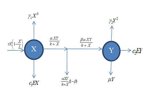
From the above flow diagram and assumptions, the resulting system is governed by the following equations:
$$ \frac {d X}{d t} = r X \left(1 - \frac {X}{L}\right) - \frac {\alpha X Y}{k + X} - \gamma_ {1} X ^ {3} - c _ {1} E X, $$ $$ \frac {d Y}{d t} = \frac {\beta \alpha X Y}{k + X} - \gamma_ {2} Y ^ {2} - \mu Y - c _ {2} E Y, $$ (5) with initial conditions
$$ : X (0) \geq 0 \mathrm {a n d} Y (0) \geq 0, $$ where:
X is the Prey fish, Y is Predator fish, r is the Prey growth rate, α is the predation rate, β is the conversion rate of prey biomass to predator biomass, k is the amount of prey consume for predator half satisfaction, µ is the natural death rate of predator, E is the harvesting effort, 1γ is the death rate of prey due to toxic substance, 2 γ is the death rate of predator due to toxic substance, 1_c_ is the catchability coefficient of prey 2_c_ is the catchability coefficient of predator, u is the toxicants control variable, 1_c EX_ is the harvesting effort of prey, 2_c EY_ is the harvesting effort of predator, 3 1_X_ γ is the infection of prey fish by external toxic substance, 2 2_Y_ γ is the infection of predator fish by external toxic substance Y µ is the natural death rate of predator, is the logistic growth of prey fish, XY k X α + $$ r X \left(1 - \frac {X}{L}\right) $$ is the predation rate, XY k X βα + is the amount of prey biomass converted to predator biomass.
Model Analysis
In this section, the formulated model above (5) will be qualitatively analysed to get the dynamical features that help to understand the effects of toxic on a prey-predator system. The boundedness and the positivity of the solution will be determined.
Boundedness
In this section we show that the system (5) is bounded or well behaved by considering the following lemma.
Lemma 1
All the solutions of the system (5) which start in 2 + � are
uniformly bounded Das [4], where 2 + � are the positive real numbers.
Proof
We define the following function;
$$ W (X, Y) = X + \frac {1}{\beta} Y, \tag {6} $$
whose time derivative is $$ \frac {d W}{d t} = \frac {d X}{d t} + \frac {1}{\beta} \frac {d Y}{d t}. \tag {7} $$ Equations (5) are substituted to equation (7) to get $$ \frac {d W}{d t} = r X \left(1 - \frac {X}{L}\right) - \frac {\alpha X Y}{k + X} - \gamma_ {1} X ^ {3} - c _ {1} E X + \frac {1}{\beta} \left[ \frac {\beta \alpha X Y}{k + X} - \gamma_ {2} Y ^ {2} - \mu Y - c _ {2} E Y \right] $$ $$ \mathrm {o r} \quad \frac {d W}{d t} = r X \left(1 - \frac {X}{L}\right) - \frac {\mu}{\beta} Y $$ For each 0 > S we get
1 dW X S SW X r S Y dt L µ β − + ≤ − + − .
Choose $S < \min\{0, \mu\}$ such that
$$\frac{dW}{dt} = SW \leq X \left[ r \left( 1 - \frac{X}{L} \right) + S \right]$$
$$\frac{dW}{dt} + SW \leq rX \left( 1 - \frac{X}{L} \right) + XS$$ (8)
The maximum value of (8) is given by $\frac{L(r+S)^2}{2r}$
so that
$$\frac{dW}{dt} + SW \leq \frac{L(r+S)^2}{2r}.$$
Let $\frac{L(r+S)^2}{2r}$ be equal to $K > 0$.
Then
$$\frac{dW}{dt} + SW \leq K.$$ (9)
The inequality (9) is a first order differential inequality. Its solution is obtained by using Integrating factor $IF = e^{st}$.
Multiplying equation (9) by the integrating factor we get
$$e^{st} \frac{dW}{dt} + e^{st} SW \leq e^{st} K$$ (10)
Equation (10) has a solution
$$W \leq \frac{K}{S} + Ce^{-st}$$ (11)
Apply the initial conditions $W_t = W_0$ and $t = 0$ leading to $W_0 \leq \frac{K}{S} + C$, or $C = W_0 - \frac{K}{S}$.
This implies that $W = \frac{K}{S} + \left( W_0 - \frac{K}{S} \right) e^{-st}$.
As $t \to \infty$, $e^{-st} \to 0$ yielding
$$C = W_0 - \frac{K}{S}.$$
We thus find that all the solutions of the equations 5 that start in $\Box^+_2$ are confined to the region $C$, where
$$C = \left\{ (X, Y) \in \Box^+_2 : W = \left( \frac{K}{S} \right) + \varepsilon, \text{ for any } \varepsilon > 0 \right\}$$ (Das et al. 2009).
Positivity of the solution
For the model (5) to be ecologically meaningful and well posed, we need to prove that all solutions with positive initial data will remain positive for all the time $t \geq 0$.
Theorem 1
Let $X_0, Y_0 > 0$. Then the solution of the model (5) is positive for $\forall t \geq 0$.
Proof
To prove the theorem, we use all equations of the system (5) from the first equation of prey population, we have
$$\frac{dX}{dt} = rX \left( 1 - \frac{X}{L} \right) - \frac{\alpha XY}{k + X} - \gamma_1 X^3 - c_1 EX$$
or
$$\frac{dX}{dt} \leq rX \left( 1 - \frac{X}{L} \right).$$
The above equation is a non-linear differential inequality which can be solved which can be solved by using separation of variables. So
$$\frac{dX}{XL - X^2} \leq \frac{r}{L} dt,$$
which imply that
$$\frac{dX}{X(L - X)} \leq \frac{r}{L} dt,$$
which has a solution
$$\ln X - \ln(L - X) \leq \frac{r}{L} t + c.$$
Similarly
$$\ln \left( \frac{X}{L - X} \right) \leq \frac{r}{L} t + c$$
or
$$X \leq \frac{Lc}{e^{-\frac{r}{L} t}} + c$$
Apply initial conditions to (12) to get
$$X_0 = \frac{eL}{e^{-\frac{r}{L} t}} + c$$
Then
$$c = \frac{X_0}{L - X_0},$$
Substitute the value of $c$ into (12) to get
$$X \leq \frac{X_0 L}{(L - X_0) e^{-\frac{r}{L}} + X_0}.$$
As $t \to \infty$ then $e^{-\frac{r}{L}} \to 0$
Thus
$$0 \leq X \leq L.$$
Similarly, using the second equation of system (5), positivity of solutions can be established. Hence, both the solutions of the system (5) that are initiated in $\Box \frac{1}{2}$ are confined in the region confined to the region $C$, where
$$C = \{(X, Y) \in R_2^+\}.$$
**Equilibrium Points and Stability analysis**
Here we study the existence and stability of steady states. The model has four equilibrium points. These are trivial steady state $E_0$, predator free steady state $E_1$, prey free steady state $E_2$ and interior steady state $E_3$.
**Definition:**
A steady state of a system (5) is a solution $X(t) = X$, $Y(t) = Y$ where $X$ and $Y$ are solutions of the algebraic equation $f(X, Y) = 0$.
So we set $\frac{dX}{dt} = \frac{dY}{dt} = 0$ and seek for the steady state solution. The system (5) becomes
$$rX^* \left(1 - \frac{X^*}{L}\right) - \frac{\alpha X^* Y^*}{k + X^*} - \gamma_1 X^*^3 - c_1 EX^* = 0$$
$$\frac{\beta \alpha X^* Y^*}{k + X^*} - \gamma_2 Y^*^2 - \mu Y^* - c_2 EY^* = 0 \quad (14)$$
**The trivial steady state**
The trivial steady state is obtained as follows:
From equation (14), we have
$$\frac{\beta \alpha X^* Y^*}{k + X^*} - \gamma_2 Y^*^2 - \mu Y^* - c_2 EY^* = 0$$
Factor out $Y^*$ to get
$$Y^* \left[ \frac{\beta \alpha X^*}{k + X^*} - \gamma_2 Y^* - \mu - c_2 E \right] = 0.$$
Either $Y^* = 0$ or $\frac{\beta \alpha X^*}{k + X^*} - \gamma_2 Y^* - \mu - c_2 E = 0$
Substitute $Y^* = 0$ into (13) to get
$$rX^* \left(1 - \frac{X^*}{L}\right) - \gamma_1 X^*^3 - c_1 EX^* = 0$$
or
$$\gamma_1 X^*^3 + \frac{rX^*}{L} - \left(r - c_1 E\right) X^* = 0$$
Factor out $X'$ and solve for $X'$ to get
$$X^* \left[ \gamma_1 X^*^2 + \frac{rX^*}{L} - \left(r - c_1 E \right) \right] = 0.$$
Either $X^* = 0$ or
$$\gamma_1 X^*^2 + \frac{rX^*}{L} - \left(r - c_1 E \right) = 0 \quad (15)$$
So trivial steady state $E_0 \left( X^*, Y^* \right) = (0, 0)$
**The predator free steady state**
The predator free steady state is obtained by solving for $X'$ in (15).
The other
Therefore,
$$X^* = \frac{\left( -\frac{r}{L} \right) + \sqrt{\left( \frac{r}{L} \right)^2 + 4 \gamma_1 \left( r - c_1 E \right)}}{2 \gamma_1}$$
the predator free steady state
**The prey free steady state**
This steady state $E_2$ is calculated as follows:
$$E_1(X', Y') = \left( \frac{\left( -\frac{r}{L} \right) + \sqrt{\left( \frac{r}{L} \right)^2 + 4 \gamma_1 \left( r - c_1 E \right)}}{2 \gamma_1}, 0 \right)$$
From $\frac{\beta \alpha X^*}{k + X^*} - \gamma_2 Y^* - \mu - c_2 E = 0$ it follows that
$$Y^* = \frac{1}{\gamma_2} \left( \frac{\beta \alpha X^*}{k + X^*} - \mu - c_2 E \right).$$
Substitute (16) into (13) to get
$$rX^* \left( 1 - \frac{X^*}{L} \right) - \frac{\alpha X^* Y^*}{k + X^*} - \gamma_1 X^{*3} - c_1 EX^* = 0.$$
Factor out $X^*$ to get
$$X^* \left[ r \left( 1 - \frac{X^*}{L} \right) - \frac{\alpha Y^*}{k + X^*} - \gamma_1 X^{*2} - c_1 E \right] = 0$$
Either $X^* = 0$ or
$$r \left( 1 - \frac{X^*}{L} \right) - \frac{\alpha Y^*}{k + X^*} - \gamma_1 X^{*2} - c_1 E = 0.$$
When $X^* = 0$, then from (16), $Y^* = -\frac{(\mu + c_2 E)}{\gamma_2}$
Thus the prey free steady state is
$$E_2(X^*, Y^*) = \left( 0, -\frac{(\mu + c_2 E)}{\gamma_2} \right).$$
The interior steady state
The interior steady state $E_3(X^*, Y^*)$ is determined as follows:
Substitute (16) into (18) to get
$$\gamma_1 \gamma_2 X^{*4} + (\gamma_2 Y^* + 2k \gamma_1 Y^*) X^{*3} + (2k \gamma_2 \frac{R}{L} + k^2 \gamma_2 + \gamma_1 c_1 E - \gamma_2 r) X^{*2} + (\gamma_2 k^2 \frac{R}{L} + a^2 \beta + 2k \gamma_2 c_1 E + (\mu + c_2 E) - 2k \gamma_2 r) X - (k(\mu + c_2 E) + \gamma_2 c_1 E k^2 - \gamma_2 k^2 r) = 0$$
Let
$$a = \gamma_1 \gamma_2, \quad b = \frac{\gamma_2 r}{L} + 2k \gamma_1 \gamma_2, \quad c = \gamma_2 \left( 2k \frac{R}{L} + k^2 \gamma_1 + c_1 E - r \right),$$
$$d = \gamma_2 k^2 \frac{R}{L} + \alpha^2 \beta + 2k \gamma_2 c_1 E + (\mu + c_2 E) - 2k \gamma_2 r,$$
$$e = -\left( k(\mu + c_2 E) + \gamma_2 c_1 E k^2 - \gamma_2 k^2 r \right),$$
$$a X^{*4} + b X^{*3} + c X^{*2} + d X^{*} - e = 0$$
Equation (20) is very difficult to solve. With help of Mathematica 9.0, the roots of (20) which are the interior steady state $E_3(X^*, Y^*)$ can be estimated by
$$rX^* \left( 1 - \frac{X^*}{L} \right) - \frac{\alpha X^* Y^*}{k + X^*} - \gamma_1 X^{*3} - c_1 EX^* = 0$$ and
$$\frac{\beta \alpha X^* Y^*}{k + X^*} - \gamma_2 Y^{*2} - \mu Y^* - c_2 EY^* = 0$$
when $X^*$ and $Y^*$ are non-negative and roots of equation (20) are defined.
Stability of the of the Equilibrium Points
We study the stability of each equilibrium point by first computing the Jacobian matrix corresponding to the model equation calculated at each steady state.
Let
$$f = rX \left( 1 - \frac{X}{L} \right) - \frac{\alpha X Y}{k + X} - \gamma_1 X^3 - c_1 EX$$ and
$$g = \frac{\beta \alpha X Y}{k + X} - \gamma_2 Y^2 - \mu Y - c_2 EY.$$
Then the Jacobian of the function $f$ and $g$ is given by
$$J(X, Y) = \begin{pmatrix} \frac{\partial f}{\partial X} & \frac{\partial f}{\partial Y} \\ \frac{\partial g}{\partial X} & \frac{\partial g}{\partial Y} \end{pmatrix}$$
$$J(X, Y) = \begin{pmatrix} r - \frac{2rX}{L} - \frac{\alpha Y k}{(k + X)^2} - 3\gamma_1 X^2 - c_1 E & -\frac{\alpha X}{k + X} \\ \frac{\beta \alpha Y k}{(k + X)^2} & 2\gamma_2 Y - \mu - c_2 E \end{pmatrix}.$$
The trivial steady state $E_0(X^*, Y^*) = (0, 0)$.
$$E_0(X^*, Y^*) = (0, 0).$$
The Jacobian (21) at trivial steady state becomes
The characteristic equation can be determined by
0 (0,0) 0 ( ) r c E E c E µ $$ \mathbf {J} E _ {0} (0, 0) = \left( \begin{array}{c c} r - c _ {1} E & 0 \\ 0 & - \left(\mu + c _ {2} E\right) \end{array} \right) $$
1 0 2 $$ \left| \mathbf {J} E _ {0} - \mathbf {I} \lambda \right| = 0 $$
$$ \det \left( \begin{array}{c c} (r - c _ {1} E) - \lambda & 0 \\ 0 & - (\mu + c _ {2} E) - \lambda \end{array} \right) = 0 $$
1
2 whose Eigen values are given by $$ \lambda_ {1} = r - c _ {1} E \mathrm {a n d} \lambda_ {2} = - \left(\mu + c _ {2} E\right) $$ The trivial steady state is stable when 1 r c E < From the result above, it can be seen that the population is at normal state at this point.
The predator free steady state
The Jacobian (21) at predator free steady state become
| r − + L | r2 +4γ (r−c E) L 1 1 |
|---|
∗ ∗ γ
| r − + L | r2 L +4γ 1(r−c 1 E) |
|---|
J
βα γ µ γ ( )
2 $$ A = r - L \sqrt {\frac {r ^ {2}}{L ^ {2}} + 4 \gamma_ {1} \left(r - c _ {1} E\right)} \mathrm {a n d} $$ where
2 r r r c E L L B γ $$ ? = \frac {\frac {- r}{L} + \sqrt {\frac {r ^ {2}}{L ^ {2}} + 4 \gamma_ {1} (r - c)}}{A _ {x}} $$
4 ( ) . 4
1 1 2 γ
1 The characteristic equation of the predator free steady state is given by rA A r B c E L kL A α λ γ γ + − − − − + = − + − − +
2 1 or $$ \left(r + \frac {r A}{L ^ {2} \gamma_ {1}} - 3 B ^ {2} - c _ {1} E - \lambda\right) \left(\frac {\beta \alpha A}{- 2 k L \gamma_ {1} + A} - \left(\mu + c _ {2} E\right) - \lambda\right) = 0 $$ (22) whose Eigenvalues are given by $$ \lambda_ {1} = r + \frac {r A}{L ^ {2} \gamma_ {1}} - \left(3 B ^ {2} + c _ {1} E\right) $$ and $$ \lambda_ {2} = \frac {\beta \alpha A}{- 2 k L \gamma_ {1} + A} - \left(\mu + c _ {2} E\right). $$ ( ) 2 2 1 2 $$ a _ {1} = r + \frac {r A}{L ^ {2} \gamma_ {1}} \mathrm {a n d} b _ {1} = \left(3 B ^ {2} + c _ {1} E\right). \mathrm {T h e n} $$ Let 1 2 1 $$ \lambda_ {1} = a _ {1} - b _ {1} \mathrm {o r} $$ $$ \lambda_ {1} = \left(R _ {1} - 1\right) b $$ $$ \left| R _ {1} ^ {(2 3)} = \frac {a _ {1}}{b _ {1}} \right| $$
. Thus if
1 1 R < , then
1λ is negative.
(23) where
1 1
1 $$ \lambda_ {2} = \frac {\beta \alpha A}{- 2 k L \gamma_ {1} + A} - \left(\mu + c _ {2} E\right) $$ From ( ) 2 2 1 2 A a kL A βα $$ = \frac {\beta \alpha A}{- 2 k L \gamma_ {1} + A} \mathrm {a n d} b _ {2} = \left(\mu + c _ {2} E\right). \mathrm {T h u s} $$ we let 2
1 2 $$ \lambda_ {2} = a _ {2} - b _ {2} \mathrm {o r} $$
$$ \lambda_ {2} = \left(R _ {2} - 1\right) b _ {2} $$
(24) If 2 1 R < then the eigenvalue 2 λ is negative So the predator free steady state is locally asymptotically stable since 1 1 R < and 2 1 R < The Prey Free Steady State $$ \left(X ^ {*}, Y ^ {*}\right) = \left(0, - \frac {\left(\mu + c _ {2} E\right)}{\gamma_ {2}}\right). $$ ( ) ( , ) 0, . c E E X Y µ γ
2 2 2 Substitute prey free steady state in the Jacobian (21) to get ( ) 0 ( ) 0, ( ) c E r c E k c E c E c E k α µ γ µ βα µ γ µ γ + + − + − = + − +
2 1 2 2 J
2 2 2 2
The characteristic equation is given by
$$\lambda_1 = r + \frac{\alpha(\mu + c_2E)}{k\gamma_2} - c_1E$$
This gives the Eigenvalues as
$$\det \begin{pmatrix} r + \frac{\alpha(\mu + c_2E)}{k\gamma_2} - c_1E - \lambda & 0 \\ -\frac{\beta\alpha(\mu + c_2E)}{k\gamma_2} & \mu + c_2E - \lambda \end{pmatrix} = 0.$$
and $\lambda_2 = \mu + c_2E$
From $\lambda_1$ we let $a_3 = r + \frac{\alpha(\mu + c_2E)}{k\gamma_2}$ and $b_3 = c_1E$.
Then $\lambda_1 = a_3 - b_3$ or $\lambda_1 = (R_1 - 1)b_3$
Where $R_1 = \frac{a_3}{b_3}$.
Thus when $R_1 < 1$ the eigenvalue $\lambda_1$ is negative. Thus the prey free steady state is locally asymptotically stable when $R_1 < 1$ and $\mu + c_2E < 0$ which means that all eigenvalues are negative.
Model with Control
In the previous section, a model without control was formulated and analysed. The boundedness, positivity, equilibrium and the local stability was discussed. In this section, a control variable is introduced in model equation (5) and the system is analysed. The main objective is to minimize toxic which affect fish population and cost of implementing control strategies. It is intended to use water hyacinth (Eichhornia crassipes (Martius) Solms-Laubach) Jafari and Trivedy [7] which is efficient in accumulating heavy metals such as lead, mercury and treat Biological and Chemical waste water [8]. Water hyacinth is a plant which is used to treat polluted water. It deals with biological and chemical wastes which are likely to affect fish population.
Water hyacinth, in other sides, can be a problem economically as it negatively affects fisheries, slow or even prevent water traffic, impedes irrigation, obstructs water ways, reduces water supply and slows hydropower generation [9].
It is assumed that the application of water hyacinth to minimize toxic in affected fish population is at a rate of $u(t)$. The model equation (5) with control variable at any time $t$ is given as
$$\frac{dX}{dt} = rX \left(1 - \frac{X}{L}\right) - \frac{\alpha XY}{k + X} - (1 - u)Y_1X^3 - c_1EX$$
$$\frac{dY}{dt} = \frac{\beta\alpha XY}{k + X} - (1 - u)Y_2Y^2 - \mu Y - c_2EY$$
(26)
with initial conditions $X(0) \geq 0$ and $Y(0) \geq 0$.
To minimize the cost of applying water hyacinth and its negative effects, we have to formulate an optimal control problem and apply Pontryagin’s maximum principle to solve it.
Optimal Control Problem
We wish to minimize the cost of applying water hyacinth, the amount of toxic in fish population, the number of water hyacinth which hinders fish growth and other negative effects. To minimize the problem, we first restrict the number of water hyacinth which is administered to water bodies (Ocean, Lake, Ponds etc.) by introducing a bound on the control as $0 \leq u(t) \leq 1$ for $t \in \left[t_0, t_f\right]$, and then form the objective function of the optimal control problem as follows:
$$J = \min_u \int_{t_0}^{t_f} \left(AY + \frac{1}{2}Bu^2(t)\right)dt$$
subject to (26) and the initial conditions. Here $A$ is the weight associated with the amount of toxicant in fish population and $B$ is the weight factor to control variable $u(t)$, $t_0$ is the initial time and $t_f$ is the final time.
Quadratic control in the objective function was chosen because we need to minimize toxic in affected fish and cost of applying water hyacinth [10]. For minimizing the toxic in fish population while minimizing control cost, we seek to find the optimal control $u^*$ such that
$$J(u^*) = \min(J(u) / \in U),$$
where $U = \{u\}$ such that $0 \leq u \leq 1$ and $t \in \left[t_0, t_f\right]$ is the control set [11].
Solving the Optimal Control Problem
In solving optimal control problem, some necessary
conditions must be satisfied. These necessary conditions come from Pontryagin’s maximum principle. The principle converts (26) and (27) into a problem of minimizing Hamiltonian function $H$ as
$$H = AY + \frac{1}{2}Bu^2(t) + \lambda_1 \frac{dX}{dt} + \lambda_2 \frac{dY}{dt},$$
(29)
Substituting (26) to (29) we get
$$H = AY + \frac{1}{2}Bu^2(t) + \lambda_1 \left[ rX(1 - \frac{X}{L}) - \frac{\alpha XY}{k+X} - (1-u)\gamma_1X^3 - c_1EX \right] + \lambda_2 \left[ \frac{\beta\alpha XY}{k+X} - (1-u)\gamma_2Y^2 - \mu Y - c_2EY \right],$$
(30)
where $\lambda_1$ and $\lambda_2$ are the adjoint variables or co-state variables. By applying Pontryagin’s maximum principle and the existence of result for optimal control, we obtain,
Proposition 1
For the optimal control $u^*(t)$ that minimizes $J(u)$ over $U$, then there exist adjoint variables $\lambda_1$ and $\lambda_2$ satisfying
$$\frac{d\lambda_1}{dt} = -\frac{\partial H}{\partial X}$$
$$= -\lambda_1 \left[ r - \frac{2rX}{L} - \frac{\alpha kY}{(k+X)^2} - 3(1-u)\gamma_1X^2 - c_1E \right] + \lambda_2 \left[ \frac{\beta\alpha Yk}{(k+X)^2} \right]$$
$$- \lambda_1 \left[ r - \frac{2rX}{L} - \frac{\alpha kY}{(k+X)^2} - 3(1-u)\gamma_1X^2 - c_1E \right] - \lambda_2 \left[ \frac{\beta\alpha Yk}{(k+X)^2} \right]$$
$$\frac{d\lambda_2}{dt} = -\frac{\partial H}{\partial Y}$$
$$= -\left[ A - \lambda_1 \frac{\alpha X}{k+X} + \lambda_2 \left[ \frac{\beta\alpha X}{k+X} - 2(1-u)\gamma_2Y - \mu - c_2E \right] \right]$$
$$- A + \lambda_1 \frac{\alpha X}{k+X} - \lambda_2 \left[ \frac{\beta\alpha X}{k+X} - 2(1-u)\gamma_2Y - \mu - c_2E \right]$$
(31)
and with transversality conditions
$$\lambda_1(t_f) = \lambda_2(t_f) = 0$$
(32)
then
$$u^*(t) = \max\{0, \min(1, \bar{u})\}$$
(33)
So to find $\bar{u}$, we apply optimality condition to (31) to Hamiltonian to get
$$\frac{\partial H}{\partial u} = Bu(t) + \lambda_1\gamma_1X^3 + \lambda_2\gamma_2Y^2.$$
(34)
We therefore solve for $u(t)$ by equating $\frac{\partial H}{\partial u} = 0$ as described by Lenhart and Workman (2007). This leads to
$$u(t) = -\frac{-\left(\lambda_1\gamma_1X^3 + \lambda_2\gamma_2Y^2\right)}{B}$$
(35)
From (33), then $\bar{u} = u(t)$. Thus the optimality condition is written as
$$u^*(t) = \max\{0, \min\left(1, \frac{-\left(\lambda_1\gamma_1X^3 + \lambda_2\gamma_2Y^2\right)}{B}\right)\}$$
(36)
Then, by standard control arguments which involves bounds on the controls, we conclude the same way as Okosun and Makinde [12] that
$$u^*(t) = \begin{cases} 0 & \text{if } \bar{u} \leq 0, \\ \bar{u} & \text{if } 0 < \bar{u}_1 < 1, \\ 1 & \text{if } \bar{u} \geq 1. \end{cases}$$
(37)
This means that the optimal control $u^*(t)$ is minimum when $\bar{u} \leq 0$, maximum when $\bar{u} \geq 0$ and $u^*(t) = \bar{u}$ when $0 < \bar{u} < 1$.
Due to prior boundedness of the state system, adjoint system, and the resulting Lipschiz structure of the ODEs, we obtain the uniqueness of the optimal control for small $t_f$.
The uniqueness of the optimal control follows from the uniqueness of the optimality system, which consist of (31) and (32) with characterization (33). There is a restriction on the length of the time interval in order to guarantee the uniqueness of the optimality system. This smallest restriction of the length on the time is due to opposite time orientations of (31) and (32); the state problem has initial values and the adjoint problem has final values [12].
Numerical Simulations for the Model with Control
In order to illustrate some of the analytical results of the study, numerical simulations for the model with control are performed using a set of reasonable values. Table 1 shows the parameter values to be used which are hypothetically chosen following the realistic ecological observations which have been suggested by previous researchers. The initial guess for prey fish and predator fish are set to be 60 and 40 respectively.
| Parameter Symbol | Parameter value | Source |
|---|---|---|
| r | 6.5 | Das [6] |
| L | 300 | Das [6] |
| α | 0.006 | Das [6] |
| k | 0.2 | Chattopadhyay [4] |
| γ 1 | 0.00005 | Das [4] |
| c 1 | 0.03 | Das [4] |
| E | 1 | Das [4] |
| β | 0.7 | Das [4] |
| γ 2 | 0.00008 | Das [4] |
| µ | 0.9 | Kar and Chattopadhyay [10] |
| c 2 | 0.04 | Das [4] |
Figure 1 below represents the graphical solutions for the state variables and the control ( ) u t .
Figure 2 shows three graphs: Prey population, Predator population and the control_u_ . From the graphs, it is observed that the prey population seems to have sharp decrease. The predator population decreases slowly to zero. This is because there is no toxic control in the whole population so the predator population may vanish. The last graph shows the control profile where 0 u = . Because of that, the prey and predator populations seem to be decreasing [13].
Figure 3 below shows the behaviour of prey predator populations with intrinsic growth change.
r=0.8 r=2.5 r=0.8 r=2.5 r=0.8 r=2.5 Figure 3: Prey population, predator population and control profile when r changes.
It is observed in figure 3 that, changing the prey growth
$$ r = 0. 8 \mathrm {t o} r = 2. 5 $$
tends to decrease both prey population and predator population. With the prey population, the graph shows that the degree of decreasing Figure 4 below shows the behaviour of the populations when predation growth rate changes.
depends on the growth rate r . It can also be seen that the predator population does not vary with the change of growth rate [14, 15, 16, 17, 18].
α=0.78 α=0.1 α=0.78 α=0.1 α=0.78 α=0.1 Figure 4: Behavioural change of prey predator populations when predation growth rate changes.
From figure 5.3, it is observed that changing of predation rate
$$ \mathrm {f r o m} \alpha = 0. 7 8 \mathrm {t o} \alpha = 0. 1 $$
affects the predator population.
The predator population decreases slowly when 0.1 r = as compared to when 0.78 r = . It is vice versa to prey population, where the lower the predation, the lower the decreasing rate and the higher the predation rate the higher the decreasing rate [19, 20, 21, 22].
Figure 5 below shows the population behaviour when death rate of prey due to toxic varies.
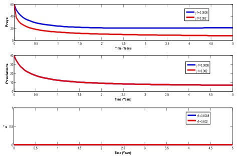
From figure 5, it is observed that, changing prey death rate
due to toxic, affects only the prey population. In prey
population, there is a sharp decrease when
$$ \gamma_ {1} = 0. 0 0 2 $$ which reflects the population dying in large numbers due to Figure 6 below shows the effect of control on prey population.
increase of toxic in the population as compared to when the
death rate is
$$ s \gamma_ {1} = 0. 0 0 0 8. $$
. The predator population is not affected by changes in 1γ [23, 24, 25, 26, 27].
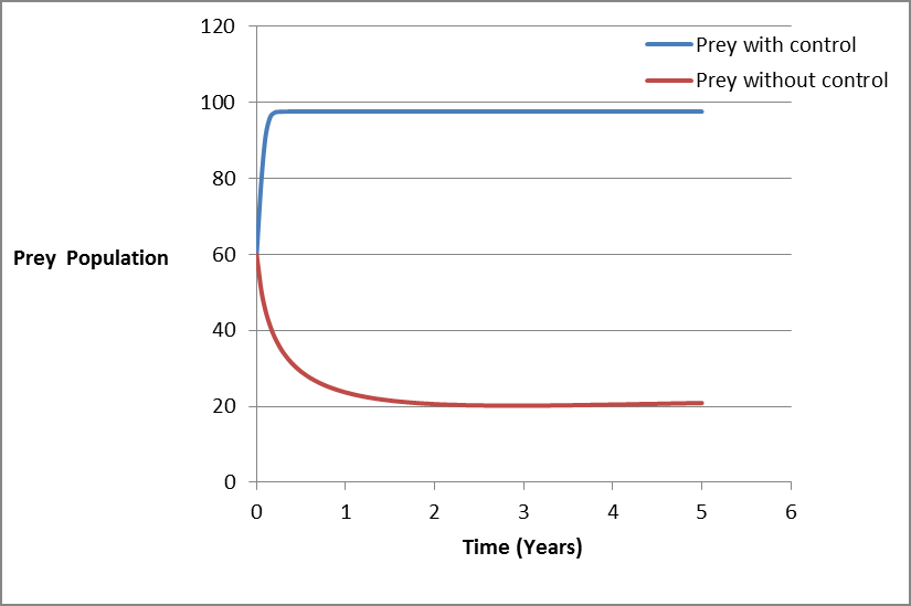
From figure 6, it is observed that prey population decreases when there is no control due to toxic in water, harvesting activities and the presence of predator. But the same population increases rapidly and when it approaches the carrying capacity it remain constant [28, 29, 30, 31, 32].
Figure 7 below shows the effect of control on predator population.
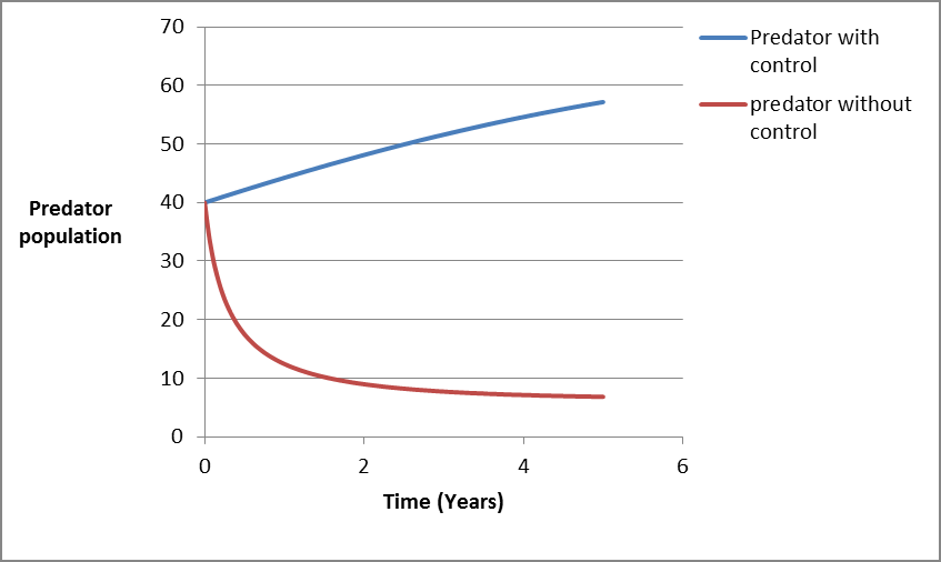
From figure 7, it is seen that the predator population decreases exponentially when there is no the control [33]. This because of the presence of toxic in water, natural death and harvesting activities which cause the population to decrease when there is no control and increasing when the control is applied to a system [34].
Summary and Conclusion
In this paper, a mathematical model for controlling toxicants in water was formulated and analysed to investigate the dynamical behaviour of the system (26). In formulating the model, harvesting effort and terms which show the effect of toxicity was introduced to both prey and predator population (fish) .Qualitative analysis was performed to the basic model (5). By applying stability theory of ordinary differential equations, four steady states were determined: trivial steady state, prey free steady state, predator free steady state and interior steady state. Model simulation revealed that application of control strategy (water hyacinth) increases fish population. It is further recommended that waste water with domestic sewage industrial effluents, thermal and radioactive pollutants may be recycled and reused to generate cheaper fuel, gas and electricity.
References
-
Samanta GP (2010) A two-species competitive system under the influence of toxic substances. Applied Mathematics and Computation 216(1): 291-299.
-
Maynard JS (1974) Models in Ecology, Cambridge University Press.
-
Chaudhuri KS, Kar TK (2003) On non-selective harvesting of two competing fish species in the presence of toxic. Ecological Modelling 161(2): 125-137.
-
Das PK, Roy S, Chattopadhyay (2009) Effect of disease- selective predation on prey infected by contact and external sources. _Indian Statistical Institute, 203 B.T._ _Road, Kolkata_ 700108_, India School of Mathematics,_ _University of Manchester, Manchester._
-
Kar TK, Chattopadhyay SK (2010) A focus on long run sustainability of a harvested prey-predator system in the presence of alternative prey. West Bengal, India.
-
Das T, Mukherjee RN, Chaudhuri KS (2009) Harvesting of prey-predator fishery in the presence of toxicity. Applied Mathematical Modelling 33(5): 2282-2292.
-
Jafari NG, Trivedy RK (2005) Environmental pollution control by using phytoremediation technology_._ Pollution Research 24(4): 875-884.
-
Jafari N (2010) Ecological and social-economic utilization of water hyacinth (Eichhorniacrassipes Mart Solm). J App Sci Environ Manage 14(2): 43-49.
-
Denny P, Masifwa WF, Twongo T (2001) The impact of water hyacinth, _Eichhorniacrissipes_ (Mart.) Solms on the abundance and diversity of aquatic micro invertebrates along the shores of northern Lake Victoria, Uganda. Hydrobiological 452(3): 79-88.
-
Kar TK, Batabyal A (2011) Stability analysis and optimal control of an SIR epidemic model with vaccination. Bio System 104(3): 127-135.
-
Makinde OD, Okosun KO (2010) Impact of Chemo- therapy on optimal control of malaria Disease with infected Immigrants. Biosystems 104(1): 32-41.
-
Okosun KO and Makinde OD (2013) Optimal control analysis of malaria in the presence of non-linear incidence rate. Appl Compt Math 12(1): 20-32.
-
Bodine NE, Gross JL, Lenhart S (2008) Optimal control applied to a model for species augmentation, Mathematical. Bio science and engineering 5(4): 669-
-
Chattopadhyay J (1996) Effect of toxic substances on a two-species competitive system. Ecological modelling 84(3): 287-289.
-
Chen F, Wu H (2009) Harvesting of a single species system Incorporating stage structureand Toxicity. Discrete Dynamics in Nature and Nature and society 290123: 16.
-
Dubey B, Hussain J (2000) Modelling the interaction of two Biological species in polluted environment. Journal of Mathematics Analysis and Application 246(1): 58-79.
-
Duncan S, Hepbun C, Papachristodoulou A (2010) Optimal harvesting on fish stocks under a time-varying discount rate. J Theor Biol 269(1): 166-173.
-
Duruibe JO, Ogwuegbu MOC, Egwurugwu JN (2007) Heavy metal pollution and human biotoxic effect. International Journal of Physical sciences 2(5): 112-118.
-
Freedman HI, Shukla JB (1991) Model for the effect of toxicant in single-species and predator-prey systems. J Math Biol 30: 15-30.
-
Gazi NH, Das K, Srinivas SAM, Srinivas NM (2011) Prey predator fishery model with stage structure in two Patchy Marine Aquartic Environment. Applied Mathematics 2(11): 1404-1416.
-
Hsui CY and Chen CC (2007) Fishery policy when considering the future opportunity of harvesting. Math Biosc 207(1): 138-160.
-
Laarabi H, Labriji El H, Rachik M, Kaddar A (2012) An Optimal control of an epidemic model with a saturated incidence rate. Non Linear Analysis, Modelling and Control 17(4): 448-459.
-
Lenbury Y and Tumrasvin N (2000) Singular Perturbation Analysis of a model for the effect Toxicants in a single- species system. Mathematical and Computer Modelling 31(5): 125-134.
-
Lenhart S, Workman JT (2007) Optimal control applied to biological models, mathematical and computation Biology series. Chappman and Hall/CRC.
-
Okosun KO, Makinde (2011) Modelling the impact of drug resistance in malaria transmission and its optimal control analysis. International Journal of Physical Sciences 6(28): 6479-6487.
-
Owa FW (2014) Water pollution: Sources, Effect, Control and management. International Letters of Natural Sciences 3: 1-6.
-
Potryagin LS, Boltyanskii VG, Gamkrelidze RV, Mishchenko EF (1962) The mathematical theory of optimal processes, Wiley, New York.
-
Samanta GP, Matti A (2004) Dynamical model of a single species system in a polluted environment. J Appl Math Comp 16: 231-242.
-
Scott GR, Sloman KA (2004) The effect of environmental pollutants on complex fish behaviour: integrating behavioral and physiological indicators of toxicity. Aquatic Toxicology 68(4): 369-392.
-
Sharma S, Samanta GP (2013) Mathematical analysis of a single-species population model in a populated environment with Discrete Time Delays. Hindawi Publishing Corporation, Journal of Mathematics 574213: 18.
-
Sinha S, Misra OP, Dhar J (2010) Modelling a predator – prey system with infected prey in a polluted environment. Applied Mathematical Modelling 34(7): 1861-1872.
-
Skiadas CH, Skiadas C (2009) Chaotic modelling and Simulation: Analysis of Chaotic Models. Attractors and Forms. CRC Press, New York, USA.
-
Straif K, Cohen A, Samet J (2013) Air pollution on cancer, International agency for research on cancer, France.
-
Ugwa KA (2012) Mathematical modelling as a tool for sustainable development in Nigeria. International Journal Academic Research Progressive Education Development 1(2): 2226-6348.
- Lessons to Learn: Trees are More than the Lungs of the World
- Community Forestry Enterprises as a Model for Sustainable Forest Development: The Case Of The "Baja Tarahumara" in Chihuahua, Mexico
- Ecological and Socio-Economic Impacts of Chromolaena odorata and Mesosphaerum suaveolens, Two Invasive Alien Species in Central and Southern Benin, West Africa
- Epigenetic Sustainability: Modeling the Human Factor as a Natural Resource through Science 4.0 and the NR3C1 Biological Pilot
- Growth-at-Risk: A Framework for Assessing Economic Vulnerability
- The Rural Territory as a Socioecological System for the Management of Public Policy for Sustainable Rural Development