Economic Limit Estimation and Production Forecasting in a Field by Using Decline Curve Analysis Method
In this paper, the decline curve analysis method is performed according to a new economic limit in a field named X (for confidential reasons). The production data are processed in EXCEL software and the forecasting is made in MBAL software by respecting the following steps: Firstly, identify the decline zone and determine the decline model on the production history, secondly estimate a new economic limit by using the actual oil price, thirdly, forecast the production and determine the reserves still recoverable and fourthly, make an economic evaluation. The interpretation of the result show that the decline zone is extended on 540 days and the decline curve showed an exponential decline by the next, the new economic limit is estimated at 381.86 Sm3/Day which allow concluding that, the life of the field X is extended from 367 days with 253,935.46 Sm3 as the ultimate recoverable reserves. By the end, these reserves can generate 11,581,676 USD as net income. The above results make it possible to understand the influence of the economic limit and by ricochet the oil price on the lifetime of field X and on its recoverable reserves. Depending on the company, the makeable net income can be set as profitable or nonprofitable. In the positive case this could allow the reopening of the field X.
Introduction
Petroleum is a naturally occurring material in the earth composed predominantly of chemical compounds of carbon and hydrogen with and without other non-metallic elements such as sulfur, nitrogen and oxygen [1, 2, 3, 4]. It is produced from oil and gas field both onshore and offshore. In the oil and gas fields the production tends to follow a profile which start by a build-up and followed by a plateau of production. After the plateau is exceeded the production decline and continues until an economic limit is reached and the field is abandoned [5, 6, 7, 8]. In the history, the low oil price has been always the main cause of oilfield abandonment [9].
The production in the field X started in February 2008 and ended in September 2016 due to the economic limit. The oil price, which is closely linked to the economic limit, is very low at this period which cause a high value of the economic limit. This can affect the lifetime and the ultimate recoverable reserves (URR) of this field. Today with a higher oil price, perform production forecasting can provide higher values of lifetime and URR of this field than the day of shutting down.
Various method has been developed to perform these forecasts like decline curve analysis method, material balance method and simulation method [10, 11, 12, 13]. Decline curves analysis is one of the most popular methods to date for evaluating the future production potential of conventional wells [14, 15]. It is the priceless method and integrated the economic limit in its forecasting. The goal of this paper is to estimate the ultimate recoverable reserves of the field X based on an updated economic limit. To achieve this, it is essential to follow the following objectives: Identify of the decline zone and determine the model of decline curve, estimate a new economic limit, determine the future production of this field and calculate the ultimate recoverable reserves and make an economic evaluation. This paper is articulated in three sections: the first section deals with the introduction, the second section presents the data, tool, methods used to achieve the various objectives, the different results obtained and the discussions. The last section is the conclusion.
Materials and Methods
The EXCEL software, MBAL software, decline curve analysis method and economic evaluation are used to attain the aims of this paper. The daily production history of the field X is presented in (Figure 1).
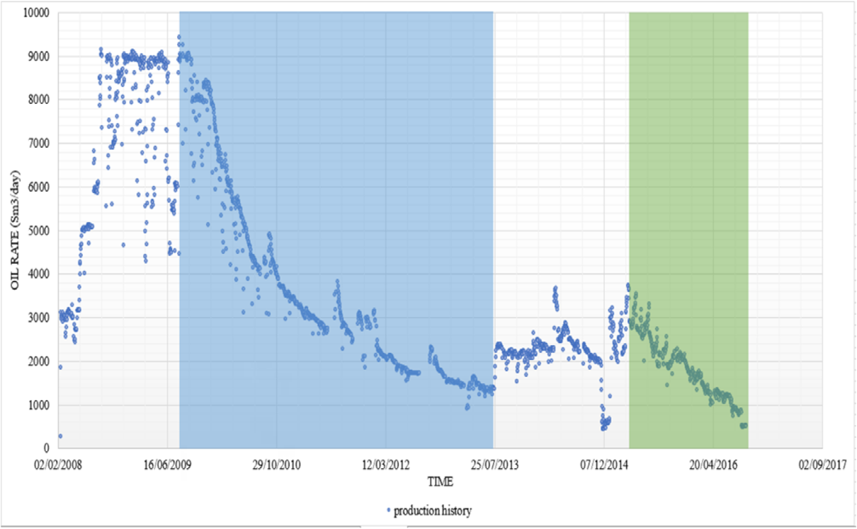
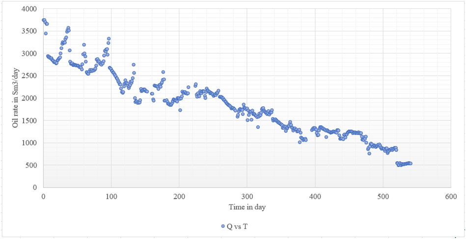
The two majors decline zones can be identify in the production history as shown in Figure 1. The first and largest decline zone begins from 10 August 2009 to about 20 July 2013. But the production rate restarts to increase and reaches a new peak of production which marks the beginning of a new decline. The second decline zone begins from the 26 April 2015 and ends the 16 September 2016. This decline represents the last until the end of the production and then is the one which will be used to proceed the decline curve analysis (Figure 2) illustrates the selected decline zone.
Results
Figure 3 shows the plot of Log of production rate (q) versus time and the plot of cumulative produced (Np) versus Log(q).
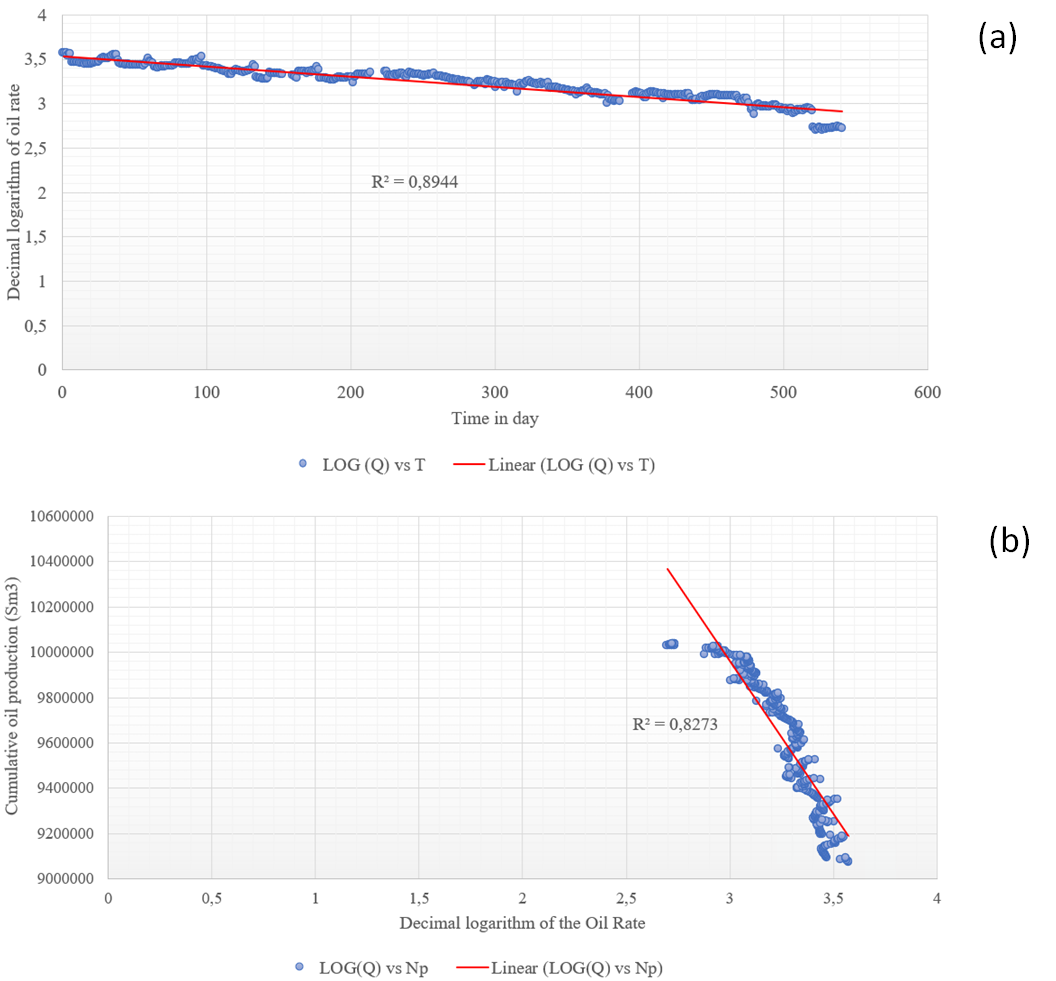
From Figure 3(a), a linear trend can be observed while in the Figure 3(b) a cocave trend can be observed. According to the litterature, the decline model is exponential with the decline exponent at b = 0. Table 1 shows the economic limit and the Brent crude oil price in September 2016 used to calculate the cost of production at this period.
| 530.27 Sm³/day | 3,335.031 STB/day | |
|---|---|---|
| Oil Price In Sept 2016 | 46.57 USD/bbl | |
| Cost Of Production In 2016 | 155,312.4 USD/day | |
| Cumulative Inflation Rate | 0.1375 | |
| Cost Of Production In 2021 | 176,667.9 USD/day | |
| Actual Oil Price | 73,56 USD/bbl | |
| New Economic Limit | 3,818,6777 Sm³/day | 2,401,684 STB/day |
Table 1: Data needed in the determination of the new economic limit.
The new economic limit is calculated by using the actual oil price (2 September 2021) and the value of the cost of production in 2021. The value of this cost in 2021 is a function of the cumulative inflation rate between 2016 and 2021. These data are also shown in (Table 1). The decline zone has been identified and the decline model known as exponential and with the economic limit of 381.87 Sm3/day, the prediction can be done. The production history used for the prediction and the production forecasted by using MBAL software are reported in (Figure 4).
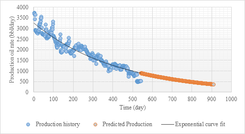
The plot of the oil production rate as function of time t is shown in Figure 4. According to the prediction, the new economic limit is reached in November 2017 precisely on November 08 and moreover, any production below this limit will no longer be considered profitable. The life of the field is now extended to about 367 days or one year. After the prediction is finished in the MBAL software, the cumulative production and the oil rate from the prediction are obtained. These data can be plot against the time in a cartesian graph as shown in Figure 5.
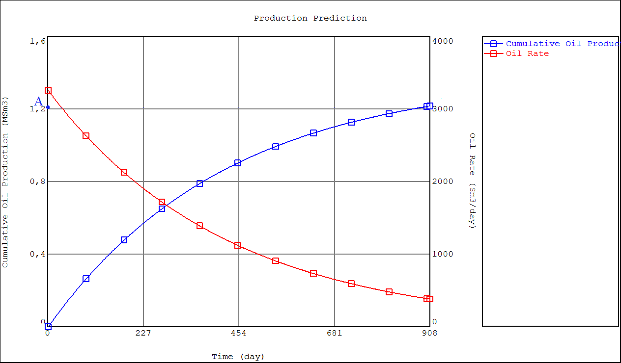
The cumulative production at the end of the prediction is also represented in (Figure 5) by the point A which is also called the estimated ultimate recovery and its value is 1,217,798.16 Sm3. The cumulative oil production at the end of the production history is already known and its value is 963,862.7 Sm3. A simple subtraction is made between these two values in order to determine the URR and its value is reported in Table 2.
| Cumulative Oil Production | 963,862.7 Sm3 | |
|---|---|---|
| Estimated Ultimate Recovery | 1,217,798.16 Sm3 | |
| Ultimate Recovery Reserves | 253,935.46 Sm3 | |
| Ultimate Recoverable Reserves | 15,97,078 | Bbl |
| Cost of Production in 2021 | 1,76,668 | USD/Day |
| Actual Oil Price | 74 | USD/STB |
| Time | 367 | Day |
| Expense | 6,48,37,109 | USD |
| Revenue from Oil Sell | 11,74,81,089 | USD |
| Taxes | 78 | % |
| Net Income | 1,15,81,676 | USD |
Table 2: Economic evaluation of the possible net income.
The evaluation of the net income is resumed in Table 3 which contains the revenue made by selling the URR and the expenses made to produce it. It contains also the value of taxes applied on the gross income (revenue – expenses) in the oil and gas sector in the region where is located the field X.
Discussion
This paper has the aim of estimate the URR of the Field X based on an updated economic limit by performing the decline curve analysis on the production data. This analysis made it possible to highlight for the field X: An exponential decline model which is the general case of reservoir with no water drive as primary recovery mechanism. This can be confirmed by the company in charge of the field and its partner which conclude that the reservoir has no or very low aquifer. After the prediction, the lifetime of the field X is extended from about one year and the recoverable reserve obtained is 253,935.5 Sm3 according to the new economic limit of 381.86 Sm3. The net income which can be made from this volume is 11,581,676 USD. This value is non-negligible when these values are for a single well for only one year of production. Based on the company policy and on its size, this economic evaluation can be considered as profitable or non- profitable. The company in charge of the field, despite the growth of the oil price, kept the field closed. This is because made their analysis and included economic parameters which fit with their size and policy. But for a smaller company, the reopening of this field can be economically profitable. The well was abandoned for five years and this could cause damage of the formation and the subsurface equipment. The irregularity in the reservoir pressure and the oil rate could be observed as well as a drop of the well deliverability. Also, the assumption made on the factors that controlling the past production which must continue in the future can influence the results by causing an overestimation of the recoverable reserves. A better understanding of these parameters will allow performing a better estimation of these reserves.
Conclusion
In conclusion, the purpose of this paper was to determine the ultimate recoverable reserves of the field X based on a new economic limit by the decline curve analysis method. By applying this method on the production data by using EXCEL software and MBAL software, different results were highlighted as a decline zone from one year long at the end of the production history, the exponential model as the exponential decline model, an extended lifetime of the field from about one year, an ultimate recoverable reserves of 253,935.5 Sm3/Day with respect to the new economic limit of 381.86 Sm3and a net income of 11,581,676 USD can be made. This paper was able to demonstrate that abandoned field X can still be reopened if the factors that caused its closure improve, in particular the economic factors. This paper is limited by some major factors which are firstly, the assumption that the past production trends and their controlling factors will continue in the future which means that any changes in the recovery method or in the production facilities can influence directly on the prediction. Secondly, the economic limit does not take into account future variations in the oil price and the inflation rate. So, this paper can be further improved by performing a material balance analysis and by making a deep analysis of economic parameters to accredit the results obtained.
References
-
Harry D (2017) Practical Petroleum Geochemistry for Exploration and Production.
-
Desorcy GJ (1979) Estimation methods for proved recoverable reserves of oil and gas. World Petroleum Congress.
-
Economides MJ, Boney C (2000) Reservoir Stimulation in Petroleum Production. Reservoir Stimulation, pp: 1-30.
-
Guo B, Lyons WC, Ghalambor A (2007) Petroleum Production engineering a computer-Assisted Appraoch, pp: 288.
-
John RF, Richard LC (2017) Introduction to petroleum engineering. Petroleum engineering.
-
John S (2018) Forecasting Oil and Gas Producing for Unconventional Wells 2nd (Edn.). Petro. Denver.
-
Boyun G, William C, Ali G (2017) Petroleum Production Engineering. Elsevier Science & Technology.
-
Bellarby J (2009) Well completion design, first edition, Elsevier, Amsterdam, Nertherlands: 304-367.
-
William C, Gary J (2005) Standard Handbook of Petroleum & Natural Gas Engineering. 2nd (Edn.), Elsevier.
-
Abdus S, Ghulam M (2016) Reservoir engineering: The fundamentals, simulation, and management of conventional and unconventional recoveries,
-
Hsu CS, Robinson PR (2019) Petroleum Science and Technology. 1st (Edn.). Chemistry and Materials Science, pp: 489
-
Jahn F, Cook M, Graham M (2003) Hydrocarbon Exploration and production. 2nd (Edn.). Developments In Petroleum Science pp: 55.
-
Arli SM (2001) Estimation and classification of reserves of crude oil, natural gas, and condensate. Richardson: AIME.
-
Tarek H (2019) Analysis of decline and types curves, Elsevier, Cambridge.
-
Arps JJ (1945) Analysis of Decline Curves, Transactions of the American Institute of Mining, Metallurgical and Petroleum Engineers 160(1): 228-247.
- Lessons to Learn: Trees are More than the Lungs of the World
- Community Forestry Enterprises as a Model for Sustainable Forest Development: The Case Of The "Baja Tarahumara" in Chihuahua, Mexico
- Ecological and Socio-Economic Impacts of Chromolaena odorata and Mesosphaerum suaveolens, Two Invasive Alien Species in Central and Southern Benin, West Africa
- Epigenetic Sustainability: Modeling the Human Factor as a Natural Resource through Science 4.0 and the NR3C1 Biological Pilot
- Growth-at-Risk: A Framework for Assessing Economic Vulnerability
- The Rural Territory as a Socioecological System for the Management of Public Policy for Sustainable Rural Development