Reassessing Baldus Study Data
Four percent of Georgia homicides in the late 1970s, the time frame of the Baldus Study, received death sentences. The rate of death sentences for White defendants was either 4% or 6%, depending on whether the victim was Black or White. In contrast, the rate of death sentences for Black defendants was either 1% or 28%, depending on the same. Baldus adjusted the data for myriad factors and concluded that there was race-of-victim bias but not race-of-defendant bias. Yet he added up the victims of each race regardless of who killed them and added up the defendants of each race regardless of who they killed. This conclusion has been taken as a starting point for many subsequent logistic regression race bias studies. If instead one asks which of the four unadjusted defendant-victim race categories B-B, B-W, W-B, and W-W have the most deviation from the 4% mean, it is the Black defendant groups, B-B and B-W, that account for almost all the error (96%). For these Black defendants, then, there was an equal protection problem in the Baldus data that went unaddressed in his Study.
Introduction
David C. Baldus and his team were pioneers in both statistics and death penalty studies with their Charging and Sentencing Study (“CSS”) [1], an early logistic regression study of race in which adjusted data, weighing hundreds of circumstances, found that race itself was among the very best predictors of a death sentence [2].
It was a sharp rebuke to the U.S. Supreme Court that reinstated the death penalty with its 1976 Gregg decision. The Court felt that aggravation-to-mitigation balancing, akin to cost-benefit analysis, could repair the lack of actus reas comparison tools in the previous legal structure for judging which murders were worst.
The study concluded that the race of the victim, but not the race of the defendant, plays a substantial part in determining whether a defendant receives a death penalty, with the chance of a death sentence being 4.3 times greater if the victim is white. Baldus’s work is indeed a finely detailed view of the trees in the death penalty woods, but the conclusion does not comport with the facts of the forest.
Emerging from the complexity of their approach, the conclusion transgresses two bedrock principles of measuring for randomness: the elemental fixedness of the four suspect- victim race categories in the data, and the operation of testing any sample against the whole of the population from which it is drawn.
An Overview of late 1970s Georgia: Homicides and Death Sentencing
During the 1973-1979 period of the Baldus Study, the FBI documented a total of 3,254 “cleared” (i.e., race- identified) homicides [3]. The unadjusted race data shows nearly all (93%) were intra-racial, with just over twice as many Black-on-Black (B-B) as White-on-White (W- W) homicides. Only seven percent were inter-racial, with just over thrice as many B-W homicides as W-B. Just three homicides (0.1%) were race-identified but lacked either a suspect or victim that was Black or White, and these incidents were set aside.
Four percent of all these homicides ultimately received a death sentence. White defendants were close enough to 4% (W-B=3.6% and W-W=6.4%) for their error to not be statistical outliers, while error with Black defendants were each far enough from 4% (B-B=0.8% and B-W=28.0%) to be statistical outliers, termed by statisticians to be statistically “significant”. This larger distance from the mean of the Black defendant death sentenced cases is the central issue of this paper. See the schema on the next page (Figure 1).
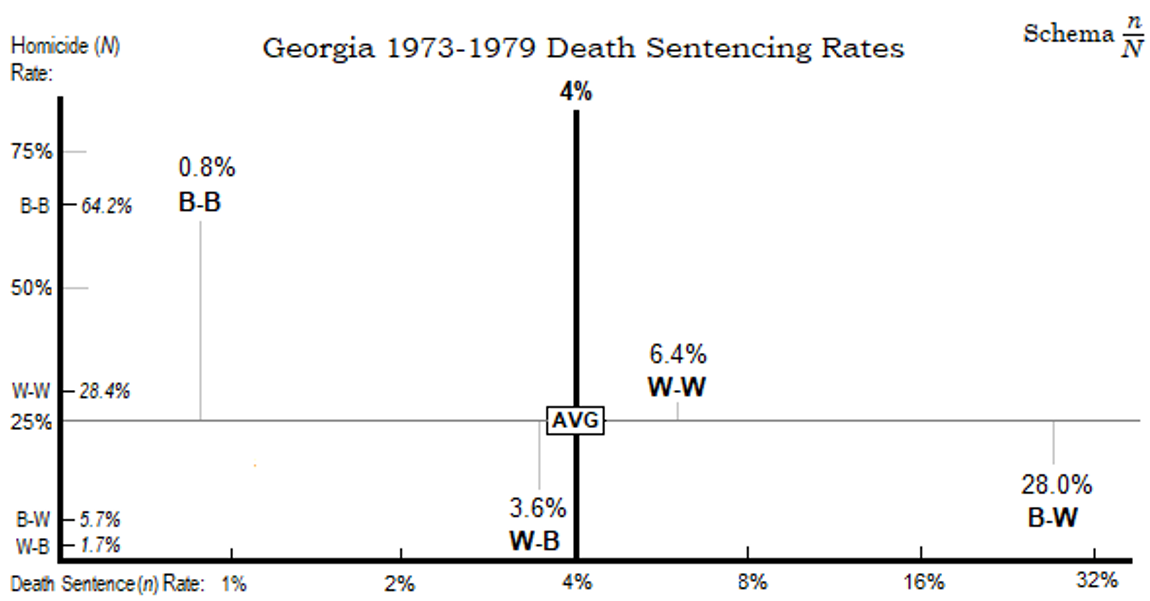
The above Schema n/N (sample divided by population) calls for some close observation and discussion.
On the schema, the physical distance of each race category name (left to right: B-B, W-B, W-W, and B-W) from AVG at the confluence of the two “means” (averages) is a good approximation of each category’s statistical error. The schema shows that the Black defendant categories B-W and B-B are each further from AVG than the White defendant categories W-B and W-W.
The left axis shows ticks of the frequency of cleared homicides (the population) for each race category, totaling 100%. The bottom axis shows the frequency of the death sentences (the sample) for each category on a log base 2 scale, where percentage doublings are equidistant.
The Problem
The principal problem with the Baldus Study is that it combined the data, not the data error (defined as the statistical deviation from the mean), of pairs of the four offender/victim race categories for analysis, making a “spurious cancellation” [4] that obscures the clearer view in Schema n/N of where the error lies. In fact, B-W data error combined with any other race category would overwhelm the error of whatever pair is left.
Baldus focused on the two categories on the right versus the two on the left, concluding there was race-of-victim but not race-of-defendant bias. Yet it is plainly visible that combining the minus and the plus of B-B and B-W data in a black defendant pairing wipes away the two poorest fits among the four race categories. It is also observable, looking only at race-of-victim pairs, that W-B lack of significant error dilutes B-B significant error, just as W-W lack of significant error dilutes B-W significant error. The effect is to negate the primacy of black defendant error.
Why Combine Categories?
There may have been compelling legal reasons to combine the data. Mixing the four race categories into pairs, rather than measuring them separately against the mean, reveals a simple and easily grasped race-of-victim bias. Many other practicalities could have led to seeking the simplest of answers.
On the other hand, when the differences between observed and expected counts of each suspect-victim category are first squared – making all error positive, whether undershoot or overshoot – and then divided by the expected count in order to temper the squared result with effect size, the least squares method has been applied and the spurious cancellations have been avoided. This is chi- squared testing.
Why Chi-Squared Goodness-of-Fit Testing is Appropriate
Are death-sentenced cases chosen from the pool of homicides in a racially neutral way?
Chi-squared testing has been used for over 120 years to answer such questions throughout the social sciences because it is relatively easy to measure and understand, with long-established lookup tables covering all reasonable probabilities. For most social science research, it is common to set the critical value at two standard deviations (sigmas) from the mean, marking a 95% probability of error as the point at which the statistic can be considered significant (unlikely to be random).
With this inquiry, since the population (the homicide count) is reported openly to the FBI and is thus well-known, and so too is the sample (the count of defendants sentenced to death), the original Pearson goodness-of-fit (one way) test, set to a critical value at its most stringent significance level of three sigmas (99.7%), is an appropriate way to test this sample data against its population for randomness (results to follow).
The Population: 3,254 Homicide Incidents
The Population of Georgia homicides from April 1973 through the end of 1979 (the time and place of the Baldus Study), a total of 3,254 cleared homicides, comes from the Murder Accountability Project file UCR65_21 of the FBI’s Uniform Crime Reports of homicide clearances. A cleared homicide is one in which at least one suspect has been arrested or identified for arrest. The UCRs do not include race data.
Race data on cleared suspects and victims is only available starting in 1976, with the FBI’s Supplemental Homicide Reports (SHRs). However, knowing the number (3,254) of cleared homicides in the whole period, we can apply the race category rates 1976-1979 to the pre-SHR period – there is no other known way to get the homicide race rates (note that 1976-1979 percentage race category distribution is nearly identical to that of the four year period 1980-1983) [5].
| Population (N) | B-B | B-W | W-B | W-W | Total |
|---|---|---|---|---|---|
| Homicide ID Count | 2,089 | 186 | 55 | 924 | 3,254 |
| Percent | 64.20% | 5.70% | 1.70% | 28.40% | 100% |
Table 1: The population counts and percents below are the 1976-1979 frequencies prorated to the UCR homicide total of 3,254.
The Sample: 130 Death-Sentenced Cases
The Sample of this inquiry is the number of cases receiving a death sentence in the Baldus Study time frame.
The original Baldus numbers have been very slightly amended by the recent study of Phillips and Marceau [6] that found a few corrections.
| Sample (n) | B-B | B-W | W-B | W-W | Total |
|---|---|---|---|---|---|
| Death Sentence Count | 17 | 52 | 2 | 59 | 130 |
| Percent | 13.10% | 40.00% | 1.50% | 45.40% | 100% |
Table 2: Death Sentence Count and Percent.
The Homicide-to-Death-Sentence Goodness-of- Fit Test
The data in Table 1 and Table 2 are used in the Pearson Chi-Squared Test performed below in Table 3. Each race category Homicide frequency percentage is multiplied by the total of 130 death-sentenced cases to derive its Expected value, for comparison to its Observed count. The race category n/N percentages from the schema on the second page are bolded. Variable numbers are rounded to the nearest integer.
| Homicide-to-Death | B-B | B-W | W-B | W-W | Total |
|---|---|---|---|---|---|
| Homicide Incidents (N) | 2,089 | 186 | 55 | 924 | 3,254 |
| Homicide frequency | 64.20% | 5.70% | 1.70% | 28.40% | 100% |
| O: Observed DS Count (n) | 17 (0.8% of N) | 52 (28.0% of N) | 2 (3.6% of N) | 59 (6.4% of N) | 130 (4.0% of N) |
| Death Sentence frequency | 13.10% | 40.00% | 1.50% | 45.40% | 100% |
| E: Expected DS (Hom freq *n) | 84 | 7 | 2 | 37 | 130 |
| Observed – Expected (O−E) | -67 | 45 | 0 | 22 | 0 |
| Pearson chi-squared test (χ²) for goodness-of-fit: | |||||
| Formula: χ² = ∑ (O − E)²/E | (-67²/84)=↓ | (45²/7)=↓ | (0²/2)=↓ | (22²/37)=↓ | -- |
| Sum, 4 race cats χ² = total χ² | 53 | 286 | 0 | 13 | 352 |
| Percentage of total χ² | 15% | 81% | 0% | 4% | 100% |
Table 3: The critical value marking significance at the 3 sigma level is χ² >14.16 (df=3, p-value <.0027). Only B-B and B-W have
Ratio data of black defendant Observed death sentences to their Expected count are shaded to emphasize their extreme nature (for B-B, 17 to 84 is a ratio of 1 : 5, and for B-W, 52 to 7 is a ratio of 7 : 1).
The Primacy of B-W Error
Each measure of four race category errors is sui generis. However, if one still wanted to combine them into pairs after squaring and testing the statistical deviation from the mean, here is how that would play out: • Race-of-defendant error: Black defendant error = 96% (81%+15%) of χ², 24 times white defendant error. • Race-of-victim error: White victim error = 85% (81%+4%) of χ², six times black victim error. • Inter- vs. intra-race error: Cross-race error = 81% (81%+0%) of χ², four times intra-race error.
B-W error dominates all pairings, calling into question the utility of examining pairs of the four race categories, even after squaring the error to avoid spurious cancellations.
Overview of All Samples
Below is Table 4, a table of different sample (n) race- category percentages divided by that of its homicide population (N). These comparisons [7] are the root Observed minus Expected residuals for testing.
| Category | Race Category Percentages | Sample / Population Percent | B-W vs. Not B-W (All Others) | |||||||
|---|---|---|---|---|---|---|---|---|---|---|
| n | B-B | B-W | W-B | W-W | n/N - All | n/N - B-W Only | B-W# | Not B-W# | Not B-W % | |
| N: Cleared Homicides | 3254 | 0.64 | 0.06 | 0.02 | 0.28 | -- | -- | 186 | 3068 | 0.94 |
| Baldus Universe Cases | 2484 | 0.58 | 0.09 | 0.02 | 0.3 | 0.76 | 1.32 | 233 | 2251 | 0.91 |
| Murder Indictments | 2343 | 0.58 | 0.1 | 0.02 | 0.3 | 0.72 | 1.24 | 231 | 2112 | 0.9 |
| Guilt at Murder Trial | 606 | 0.38 | 0.21 | 0.02 | 0.38 | 0.19 | 0.7 | 130 | 476 | 0.79 |
| All Multiple Defendants | 509 | 0.41 | 0.27 | 0.01 | 0.31 | 0.16 | 0.73 | 135 | 374 | 0.73 |
| Extra Defendants | 305 | 0.39 | 0.28 | 0.01 | 0.32 | 0.09 | 0.46 | 86 | 219 | 0.72 |
| Death Penalty Trials | 253 | 0.17 | 0.37 | 0.02 | 0.44 | 0.08 | 0.5 | 93 | 160 | 0.63 |
| Death Sentences | 130 | 0.13 | 0.4 | 0.02 | 0.45 | 0.04 | 0.28 | 52 | 78 | 0.6 |
| Executions | 25 | 0.08 | 0.48 | 0 | 0.44 | 0.01 | 0.06 | 12 | 13 | 0.52 |
Table 4: Difference between the Race Category Percentages, Population Percent and B-W vs. Not B-W.
As the sample sizes are reduced towards death, the differences in the progression of each race category are quite visible. B-W is dramatically increasing its representation in the whole (see the right-most columns that compare B-W to the other three categories) as the n sample size decreases.
The 2,343 Murder Indictments Sample
The Baldus Study’s “universe of cases” [8] (second row above) is not the homicide population. It is a sample, all the convictions of murder or voluntary manslaughter conclusively derived from the homicide population. All homicide case convictions of charges less than manslaughter, and also all homicides that were dismissed, found not guilty, or never charged, were removed from the cleared homicide population.
Instead, the murder indictments sample below is the count of all capitally-indicted cases, leaving out only the 141 cases from the Baldus universe that were always manslaughter cases, never indicted for murder.
| Indictments Sample | B-B | B-W | W-B | W-W | Total |
|---|---|---|---|---|---|
| Homicide Incidents (N): | 2,089 | 186 | 55 | 924 | 3,254 |
| Murder Indictments (n) | 1,347 | 231 | 55 | 710 | 2,343 |
| Expected Cases (N rate) | 1,504 | 134 | 40 | 665 | 2,343 |
| Observed − Expected | -157 | 97 | 15 | 45 | 0 |
| χ² of Indictments Sample | 16 | 71 | 6 | 3 | 96 |
| Percentage of total χ² | 17% | 74% | 6% | 3% |
Table 5: Showing the Indictments Sample.
Note that getting from the population of cleared homicides to the sample of murder case indictments means losing 742 B-B counts, but adding 45 B-W counts. The increase in B-W murder case convictions (shown in the B-W Only column of Table 4, it is 124% of the number of homicide incidents) must be coming from extra and uncleared offenders. This is an example of how B-W case totals can increase and even surpass its SHR population count during the post-filing period after the homicides have been reported to the FBI.
The Three Mid-Level Samples
In these three samples, the B-W percentage jumps up toward the neighborhood of the W-W percentage, while the B-B percentage falls beneath that range, a range from 22% to 44% for these three sample counts (remember here that the homicide counts were B-B=2,089, B-W=186, and WW=924) [9]:
| Mid-Level Samples | n | B-B | B-W | W-B | W-W |
|---|---|---|---|---|---|
| Guilt at Murder Trial Count | 606 | 0.38 | 0.22 | 0.02 | 0.38 |
| Multiple Offender Count | 509 | 0.41 | 0.27 | 0.01 | 0.31 |
| Penalty Trial Count | 253 | 0.17 | 0.37 | 0.02 | 0.44 |
| Guilt at Trial Sample | B-B | B-W | W-B | W-W | Total |
| Homicide Count (N) | 2,089 | 186 | 55 | 924 | 3,254 |
| Guilt at Murder Trial (n) | 232 | 130 | 14 | 230 | 606 |
| Expected Cases (N rate) | 389 | 35 | 10 | 172 | 606 |
| Observed − Expected | -157 | 95 | 4 | 58 | 0 |
| χ² of Advanced Sample | 63 | 263 | 1 | 20 | 347 |
| Percentage of χ² | 18% | 76% | 0% | 6% |
Table 6: Guilt at Trial Sample.
The 606 Guilt at Murder Trial Sample
This Baldus Study sample is of murder cases found guilty at trial [10]. The number of B-W cases thus advancing to penalty phase consideration is only 56 fewer than the homicide count of such incidents reported to the FBI. Because of this, the χ² of B-W error measures enormously out-of-line.
The 509 All Multiple Offenders Sample
This sample includes both the lead offender assigned to the multiple Incident ID and the extra offenders from those incidents, counted separately in the source data. Though similar to the Guilt at Murder Trial sample results, the W-W multiple offenders are not over-populated here. Both white defendant categories make no percentage contribution whatsoever to another highly error-filled chi-squared statistic.
| Multiple Offenders | B-B | B-W | W-B | W-W | Total |
|---|---|---|---|---|---|
| Homicide Count (N) | 2,089 | 186 | 55 | 924 | 3,254 |
| Multiple Offenders Count (n) | 207 | 135 | 7 | 160 | 509 |
| Expected Cases (N rate) | 327 | 29 | 9 | 144 | 509 |
| Observed − Expected | -120 | 106 | -2 | 16 | 0 |
| χ² of Multiple Offs Sample | 44 | 386 | 0 | 2 | 432 |
| Percentage of χ² | 10% | 90% | 0% | 0% |
Table 7: Sample of Multiple Offenders.
Combining the 204 Lead Offenders in Multiple Suspect Homicides with 305 Extra Offenders
These two sub-groups of the All Multiple Offenders sample both evenly reiterate the All sample’s total percentage of χ² in their chi-squared tests. Here is the n/N percentage comparison of the 204 lead offenders in multiple offender homicide incidents; the 305 extra offenders in such incidents; and the 509 total of the two [11]. B-W% (shaded) is more than four times the average in each multiple offender group.
| Summary of Multiple Offs | B-B % | B-W % | W-B % | W-W % | Avg of All % |
|---|---|---|---|---|---|
| 204 Lead Offenders in Mult Hom IDs % | 0.04 | 0.26 | 0.05 | 0.07 | 0.06 |
| 305 Extra Offenders Only % | 0.06 | 0.46 | 0.07 | 0.1 | 0.09 |
| 509 Total Multiple Offenders % | 0.1 | 0.73 | 0.13 | 0.17 | 0.16 |
Table 8: Summary of Multiple Offs.
The 253 Death Penalty Trials Sample
This final mid-level sample is of the number of convicted murderers who had a death penalty trial. The black defendant disconnect fully emerges at this stage. Even though only 8% (186/2,275) of black defendant homicides are B-W, these cases constitute 68% (93/137) of black defendant death penalty trials.
| Death Penalty Trials | B-B | B-W | W-B | W-W | Total |
|---|---|---|---|---|---|
| Homicide Count (N) | 2,089 | 186 | 55 | 924 | 3,254 |
| Penalty Trial Count (n) | 44 | 93 | 4 | 112 | 253 |
| Expected Cases (N rate) | 163 | 14 | 4 | 72 | 253 |
| Observed − Expected | -119 | 79 | 0 | 40 | 0 |
| χ² of Penalty Trials Sample | 86 | 427 | 0 | 22 | 535 |
| Percentage of χ² | 16% | 80% | 0% | 4% |
Table 9: Death Penalty Trials.
Death Sentencing and Execution
To recap, the death sentenced cases are the core sample of this inquiry. Here is another table, now with all the sample counts (and with the Death Sentenced Cases bolded), to view again the gleaning process in context, this time featuring the ratio of Observed to Expected counts (sample to population, or n : N).
| Category | Race Category Counts | Ratio Observed : Expected | |||||||
|---|---|---|---|---|---|---|---|---|---|
| n | B-B | B-W | W-B | W-W | B-B n : N | B-W n : N | W-B n : N | W-W n : N | |
| Cleared Homicides (N): | 3254 | 2089 | 186 | 55 | 924 | -- | -- | -- | -- |
| Murder Indictments | 2343 | 1347 | 231 | 55 | 710 | 6 : 7 | 7 : 4 | 4 : 3 | 1 : 1 |
| Murder Guilt at Trial | 606 | 232 | 130 | 14 | 230 | 4 : 7 | 4 : 1 | 4 : 3 | 4 : 3 |
| Multiple Offender Count | 509 | 207 | 135 | 7 | 160 | 3 : 5 | 5 : 1 | 4 : 5 | 7 : 6 |
| Death Penalty Trials | 253 | 44 | 93 | 4 | 112 | 2 : 7 | 7 : 1 | 6 : 7 | 3 : 2 |
| Death-Sentenced Cases | 130 | 17 | 52 | 2 | 59 | 1 : 5 | 7 : 1 | 6 : 7 | 5 : 3 |
| Executed Offenders | 25 | 2 | 12 | 0 | 11 | 1 : 8 | 12 : 1 | 1 : 1 | 3 : 2 |
Table 10: Race Category counts aand Ratio Observed: Expected.
After all this culling, at execution the black defendant imbalances (shaded) take one last proportional step away from any goodness of fit, becoming downright lopsided at the point of death.
Conclusion
One need not weigh aggravators against mitigators in these Georgia murder case outcomes in order to conclude that significant race category error is consistent and specific, principally in the B-W category where the frequency of death sentencing far exceeds the expected, but also in B-B where it lags the expected.
To view these same race category frequencies as probabilities:
- For all categories, 1 in every 25 homicides gets a death penalty.
- For white defendants, 1 in every 28 W-B, and 1 in 16 W-W get death.
- For black defendants, 1 in every 123 B-B, and 1 in 4 B-W get death.
The B-W death frequency is thus 35 times B-B death frequency (28.0% / 0.8%). This black defendant race-of- victim bias is much larger than Baldus’s odds multiplier bias of 4.3 times greater for all white victim cases.
These numbers are sufficient to raise the presumption of uneven policing as a working theory to explain the data. Specifically, white suspects are investigated in a race-neutral manner, insofar as their death sentence frequency measures off without significant error regardless of who they kill. But black suspects are handled in very different ways depending upon the race of the victim: either with light disregard, leading to increasing under-representation as B-B cases progress; or else with heavy round-ups multiple suspects becoming murder case defendants for cross-interrogation purposes leading to increasing over-representation as B-W cases progress [12].
My findings dovetail with Baldus-modelled adjusted data studies that serve to discredit the common notion that more aggravation explains the higher frequency of B-W cases. It does not, when race is compared to the worst aggravators; nor can it here, where unadjusted suspect-victim race category rates are too extreme to allow any explanation that B-W crimes are more heinous (or B-B crimes less) than others.
The Department of Justice was founded in 1870 to ensure that all Americans enjoy equal protection of the laws [13]. The distance from the norm of something as essential as the application of the death penalty to black defendants is a fundamental problem [14, 15].
I leave a final word to Jim Greiner, Harvard Law School professor and a PhD in statistics, who wrote so well and so charitably on November 30, 2006 : “As part of my dissertation research, which focuses on applying a potential outcomes understanding of causation to perceptions of immutable characteristics, I am reexamining the Baldus Study data. With the benefit of 25+ years of hindsight, I have reluctantly concluded that the Study’s findings are questionable (which is different from wrong).” This paper is an effort to fully elucidate what was most questionable and problematic in the Baldus Study.
References
-
Tim Lyman is a Document Specialist in New Orleans. He was highly trained in Information Mapping to document the Shop Floor Control module of world-class manufacturing software at Cullinet in the 1980s.
-
David C. Baldus, Charles Pulaski, and George Woodworth, Comparative Review of Death Sentences: An Empirical Study of the Georgia Experience, 74 J. CRIM. L. & CRIMINOLOGY 661 (1983). https://scholarlycommons. law.northwestern.edu/jclc/vol74/iss3/2 See also their 1990 definitive Study data in Equal Justice and the Death Penalty: A legal and empirical analysis (EJDP) by Baldus, David C., https://archive.org/details/ equaljusticedeat0000bald.
-
See the Summary Table 55 (page 326) at EJDP. See also Table 52 (page 319) for the WHITEVIC factor significance peers at the largest three-sigma level (.003 or less): TORTURE, ESCAPEE, MULTSTAB, and RAPE.
-
This number of cleared homicides comes from the Murder Accountability Project at https://www. murderdata.org. MAP gives each homicide incident of the FBI’s Supplemental Homicide Reports (“SHRs”) a unique incident ID number, with the first listed offender and victim from the original SHR sequencing representing the incident. (The SHRs call suspects “offenders.”) Then, extra offenders and victims are counted in separate columns, so that the incident, offender, and victim counts of each incident are identical. This makes it much easier (if very slightly less accurate) to count race categories, relative to my Louisiana dataset with more granularity on extra offender race.
-
Steven Strogatz, from Infinite Powers, www.hmhbooks. com, page 111, Chapter 4, The Dawn of Differential Calculus : “But total error is not quite the right concept, because we don’t want the negative errors to cancel the positive ones and give the false impression that the fit has less error than it does. Undershoots are just as bad as overshoots, and both should be penalized; they shouldn’t be allowed to cancel out. For this reason, mathematicians square the errors at each point to make the negative ones become positive. That way, they can’t possibly produce any spurious cancellations. (Here’s one place where the fact that a negative times a negative is a positive is useful in a practical setting. It makes the square of a negative error count as a positive discrepancy, as it should.)…. This approach is called the method of least squares.”
-
Homicide percentage distribution 1976-79 was 64%- 6%-2%-28% for BB-BW-WB-WW. For 1980-83 it was 67-4-2-27. For the seven years 1983-1989, a decade after the Baldus Study era, it was 67-5-1-27. For all GA SHRs, 1976-2021, it was 66-7-2-25.
-
Whom the State Kills by Scott Phillips and Justin F Marceau: https://journals.law.harvard.edu/crcl/wp- content/uploads/sites/80/2020/08/08.10.2020- Phillips-Marceau-For-Website.pdf.
-
Unadjusted Baldus data used for Observed data here are from the following tables (see Appendix DOI: 10.23880/ oajcij-16000133a) in Equal Justice and the Death Penalty: Murder Indictments in Note Table 10, page 363; Guilt at Murder Trial in Table 30, page 150; and Death Penalty Trials in Table 56, page 327. Multiple and Extra Defendants apply the FBI’s SHR 1976-79 race category frequencies to the N of 3,254.
-
“The universe of cases for the CSS consists of 2,456 offenders listed in the records of Georgia’s Department of Offender Rehabilitation as having ‘date sentence began’ (usually date of arrest) after March 27, 1973, and before January 1, 1980. This population included 100 death sentences, 876 life sentences, and 1,480 manslaughter sentences.” – EJDP (p. 66, Note 10). Twenty-eight death- sentenced cases not listed by the Georgia DOR were added later, for a total universe of 2,484 convictions. In part due to conflicts in the Baldus documentation, the cleaner Indictments data of 2,343 cases from Note Table 10 is preferred.
-
My Louisiana data race percentages leveled out in the same manner when pared to cases retaining capital charges as the final charge sought. There, in a sample of 385 capital cases, B-B was 31%, B-W 32%, and W-W 35%, when the homicide pool was 63-11-23 percent across the same three categories. See Chi-Grams of Louisiana Capital Charging at https://ssrn.com/ abstract=4148636.
-
A previous version of this paper used McCleskey v. Kemp, 481 U. S. 356 (1987), a secondary source, for this data. Table 30 (see Appendix) on page 150 of EJDP, the primary source, clearly notes the 606 denominator of the table includes “all cases in the study.” There is a diagram of the group Trial/Guilty/Murder pointing to the box “Advancement to Penalty Trial” at EJDP, p. 41.
-
What is missing (since the Baldus data only included convictions) are some extra defendants. If they are from the uncleared cases, they also escape the SHR counts. In my 41%-of-Louisiana database spanning 1976-2014, fully 7.4 % of the B-W capital cases came from multiple defendants in cases that were later matched to uncleared SHR incidents (the other race categories came in only at 1.5% on this). See Chi-Grams of Louisiana Capital Charging at https://ssrn.com/abstract=4148636. In other words, the search for more prime suspects in B-W cases clearly continues vigorously after the SHR filing due dates.
-
No analysis can help much with determining mens rea (Latin for “guilty mind,” also termed “malice aforethought”), the second pillar, with aggravation (actus reas) for proof of capital murder beyond a reasonable doubt. However, seeing the unadjusted data presented here allows glimpses of how the bias works in black defendant mistreatment. A key finding from Louisiana is that B-W leads the four race categories in overcharging, a measure unavailable to Baldus because homicides that did not produce a murder conviction were never a part of the study. Overcharged cases in Louisiana are defined as first-degree murder arrests that were subsequently reduced beyond second degree and manslaughter to less than murder, or dropped. B-W led the race category frequencies in this and every other outcome category of capitally charged cases in Chi-Grams of Louisiana Capital Charging.
-
The Fourteenth Amendment (equal protection) was ratified in 1868, and the Fifteenth Amendment (prohibition of voting rights discrimination) was ratified in 1870.
-
https://blogs.iq.harvard.edu/remembering_the_1 . For Greiner’s unique effort with his mentor, the noted statistician Donald Rubin, to set up guard rails for logistic regression analyses using the Baldus Study as an example, see: https://direct.mit.edu/rest/ article-abstract/93/3/775/57960/Causal-Effects-of- Perceived-Immutable?redirectedFrom=fulltext.
- Suicide and the Emotions of Men and Women in Uniform
- The Need to Teach Research Methods to Criminal Justice Students
- Combating Cyber VAT Fraud in the EU Member States: A Comparative Study of Criminal and Criminal Procedure Law
- Cyber VAT Fraud in the EU: A Criminological Analysis
- Advancing Compassionate Justice: Redefining Victim and Offender Rights in Victimology and Penology
- The Political Economy of Preventive Justice