Dark Numbers and Herd Immunity of the First Covid-19 Wave and Future Social Interventions
he Gauss model for the time evolution of the first corona pandemic wave allows to draw conclusions on the amount of unreported cases per reported case, i.e., ”dark number” of infections, the amount of herd immunity, the used maximum capacity of breathing apparati and the effectiveness of various non-pharmaceutical interventions in different countries. In Germany, Switzerland, Sweden, and Austria the dark numbers are 8.4±4.0, 12.6±5.8, 21.8±9.1, and 8.5±5.2, respectively. Our method of estimating dark numbers from modeling both, infection and death rates simultaneously serves as important benchmark to judge on the completeness of testing large portions of the population. For countries that cannot afford the laborious, timeconsuming and costly testing our method still provides them with a reliable estimate of the fraction of infected persons. In Germany the total number of infected individuals, including the dark number of infections by the first wave is estimated to be 1.6±0.5 million, corresponding to 1.9±0.6 percent of the German population. We work out direct implications from these predictions for managing the 2nd and further corona waves.
Reinhard Schlickeiser1,2* and Martin Kröger3
Introduction
Nowadays, numerous models to predict the spread- ing of infectious diseases like Covid-19 are available, for example the actively discussed Susceptible-Infectious- Recovered/ Removed (SIR) model [1, 2, 3, 4, 5]. Many of these models are either toy models using families of functions [6, 7, 8, 9], machine learning [10, 11, 12], neural network [13, 14], transmission [15, 16], growth [17], agent-based [18], or Bayesian regression models [19, 20] or they are so complex [4, 21], by taking into account a wide range of factors, that simple predictions are not possible [22, 23]. The progression of the first Covid-19 wave is different in the countries over the world. In some countries such as Austria, Switzer- land and Italy the peak infection and death rates have already occurred [24, 25], whereas other countries such as Argentina, Bo- livia, Egypt, India, are still in the rising phase of the first wave [26].
Recently [27], we demonstrated that the proposed28 Gaussian time (t) distribution functions for the daily fatalities d(t)
2 ,max − − = (1)
t t d w d t d
max ( ) e d and the daily infections i(t)
2 ,max − − = (2)
t t i w i t i
max ( ) e i provide a quantitatively correct description for the monitored rates in 25 different countries (more countries and federal states were subsequently investigated online [28] using real-time data). The Gauss model (GM) is one of the most prominent bell-shaped case distribution functions, originally advocated by Farr [29] to describe quantitatively the time evolution of virus diseases.
In the above equations (1) and (2), t_d_,max and t_i_,max de-note the peak times of daily cases, d_max and _i_max the maximum daily values of deaths and infections, and wd and wi the half widths of the Gaussians. One has _d(td,_max + w) = d(t_d,_max)/e0.368_ d(td,_max), in particular, where _e denotes Euler’s number.
While a more detailed model with more parameters and ingredients might be able to describe the time evolution of pandemics more accurately, the required information is not available at the beginning of emerging pandemics such as Covid-19. The necessarily sigmoidal shape of the number of fatalities can, in general, be captured by an exponential daily number of cases d(t), whose argument is a polynomial [27]. The coefficient of the highest order, necessarily even, polynomial term must be negative to ensure a sigmoidal shape. The GM represents the expansion to lowest order and is for this reason the model that can make extremely early predictions, especially about the time and amplitude of the peak values. These values are sufficient to estimate amounts of equipment during peak times, while the amplitude has usually a larger error bar and allows estimating, the later, the better, quarantine and related factors. The GM also results from an agent-based model, as long as the model conditions (social distancing etc.) remain unchanged [27]. More importantly, it is a special case of the SIR model, as recently shown by Barmparis and Tsironis [5].
The Gauss model (GM) is capable to reproduce reasonably well the monitored time evolution of the Covid-19 disease [5, 6, 7, 26, 27], and even more important to make realistic pre- dictions for the future evolution of the first wave in different countries. However, due to severe non-pharmaceutical interventions (NPIs) taken in almost all countries during the corona wave, the predicted final numbers of fatalities and infected persons sometimes disagree by about 50 percent with the monitored numbers in countries where the first wave is al- most over. This should not be taken as an argument against the GM as its applications are based on the assumption that the NPIs are not changed during the whole course of the wave evolution. Therefore, the GM allows us already now to draw important clues from the first Covid-19 wave, which is the subject of this manuscript. To be specific, the GM allows estimating the number of unreported infections, the degree of herd immunity, the used maximum capacity of breathing apparati and the effectiveness of various non-pharmaceutical interventions in different countries. We work out direct implications from these predictions for managing the 2nd and further corona waves.
Methods
The GM is adjusted to reported data as follows. Equations (1) and (2) define the GM for the time evolution of daily cases, involving three parameters for both deaths and infections. These parameters are most conveniently obtained from reported numbers upon fitting the logarithms ln d(t) and ln i(t) to a simple polynomial of grade 2 in time, i.e.
ln d(t)=d_0+_d_1_t-d_2_t_2, (3) where the three polynomial coefficients _d0,1,2 are related to the parameters of the GM, because the logarithms of equations (1) and (2) are 2nd order polynomial as well. Comparing the coefficients, one obtains
2 ,max ,max 0 max 1 2 2 2 2 2 1 ln ,d , d d
t t d d d w w w = − = = (4)
d d d and similarly for the infections. In turn, we can solve the three equations (4) for the three unknowns of the GM. The parameters of the GM are then given by the fitted polynomial coefficients via
1 , , , 2 d d d d d d d e t w d d
2 0 1 2 4 1 max ,max 2 2
+ + = = =
1 , , 2 i i i i i i i e t w i i
2 0 1 2 4 1 max ,max 2 2
+ + = = = (5)
While d_max and _i_max are daily rates, _td,max, ti,max are dates, and wd, wi are durations, both dates and durations usually specified in units of days. From equations (1) and (2) one finds for the corresponding cumulative numbers of deaths D(t) and infections I(t) − = = + − = = + t t D D t dt d t w t d ∫ ,max ' ' tot ( ) ( ) 1 erf , 2 (6) d −∞ t t I I t dt i t w t i ∫ ,max ' ' tot ( ) ( ) 1 erf , 2 i −∞ respectively, in terms of the error function, where tot max tot max , d i D d w I i w π π = = (7)
denote the total number of deaths and infections, respectively. For the GM the total numbers at the end of a pandemic wave are thus proportional to the peak amplitude and peak width of the Gaussian.
From D_tot and _I_tot we obtain an estimate of the dark number of infections (number of unreported cases per reported case), if we introduce a fraction _f of seriously sick out of all infected individuals (value for f specified later in this manuscript). Dividing D_tot by _f we can then estimate total true (reported plus unreported) number of infected individuals as D I f = true tot tot (8) Consequently, the dark number of infections, i.e. the number of infected individuals unreported for each reported, is true tot tot 1 d I N I = − (9) Throughout this manuscript we introduce placeholders marked by an asterisk, such as γ∗, α∗, that characterize a possible deviation between our working assumptions and reality. The marked quantities can all be set to unity or completely ignored during reading. If some of the numbers used in this study were to be replaced by more accurate numbers in the future, the present manuscript can still be used without change. This is so, because we introduced the marked quantities. They are unity if the present assumptions apply, and can be altered, leading to new numerical values, while the equations remain valid.
Results
In 14 countries the monitored death and infections rates were of sufficient quality by April 2 to determine via the procedure described in the previous system the values of the six coefficients in (3) with 95 percent confidence for each country in our recent work [27]. From these coefficients we readily inferred according to equation (5) the best values and their 95 percent confidence errors of the only three parameters (d_max,_td,max, wd) and (i_max,_ti,max,wi) determining the Gauss functions (1) and (2). The mentioned work reported the respective death rate parameters (d_max,_td,max,w_d), determined on April 2, 2020 (results collected in the appendix), but omitted the corresponding values of the reported infections rate parameters (_i_max,_ti,max,wi).
Here we update this statistical analysis of the GM with the available monitored data until May 19, 2020. Our best fits for selected countries Germany, Switzerland, Sweden and Austria are shown in Figure 1 for the daily infection and death rates and in Figure 2 for the cumulative number of infections and fatalities. Table 1 lists the resulting best fit values for the four countries. We include the fade out time T_1% that had been defined in [27] as the date at which the number of daily infected people _d will have reduced to the level of 1% of its maximum value, and the dark number of infections Nd. As visible from Figure 1, daily fatalities are better described by gaussians than the reported daily infections, while the true daily infections can be expected to share their overall shape with the daily fatalities. This feature directly takes over to Figure 2 via equation (6), and will be discussed further below.
| Code | w i | t i,max | i /1000 max | I /1000 tot | w d | t d,max | d max | D /1000 tot | T 1% | N d |
|---|---|---|---|---|---|---|---|---|---|---|
| DEU | 19.7±0.1 | Apr-11±2 | 5.0±1.3 | 173±30 | 18.0±0.1 | Apr-19±2 | 255±80 | 8.2±2.5 | 23-May | 8.4±4.0 |
| CHE | 19.5±0.1 | Apr-06±2 | 0.8±0.2 | 28±7 | 18.9±0.1 | Apr-13±2 | 56±16 | 1.9±0.4 | 18-May | 12.6±5.8 |
| SWE | 27.5±0.2 | Apr-22±3 | 0.7±0.2 | 34±8 | 19.0±0.1 | Apr-19±2 | 115±27 | 3.9±0.7 | 20-Jun | 21.8±9.1 |
| SWE Hopkins | 26.9±0.2 | Apr-23±3 | 0.7±0.2 | 34±9 | 20.5±0.2 | Apr-25±4 | 100±50 | 3.8±1.8 | 20-Jun | 20.8±15.3 |
| AUT | 21.5±0.2 | Apr-07±4 | 0.4±0.2 | 13±3 | 18.1±0.1 | Apr-13±3 | 20±7 | 0.6±0.2 | 23-May | 8.5±5.2 |
Table 1: Best Gaussian fit parameters obtained as described in this work and their 95 percent confidence range: width _w__x_ (in
Table 1: Best Gaussian fit parameters obtained as described in this work and their 95 percent confidence range: width wx (in days), peak time tx,max, and peak amplitude x_max, with _x { , } d i ∈ , calculated on May 19, 2020, for reported infected (x = i) and deceased (x = d) as well as the resulting estimates for total number of fatalities _D_tot and infections _I_tot according to equation (6), dark number _N_d of infections according to (11) with α∗ = γ∗ = 1, and fade-out time _T_1%. Data for Germany (DEU), Switzerland (CHE), Sweden (SWE) and Austria (AUT). Data for Sweden differs depending on the data source. While the first dataset is from the public health agency from Sweden [25], the 2nd was collected by the John Hopkins University [30].
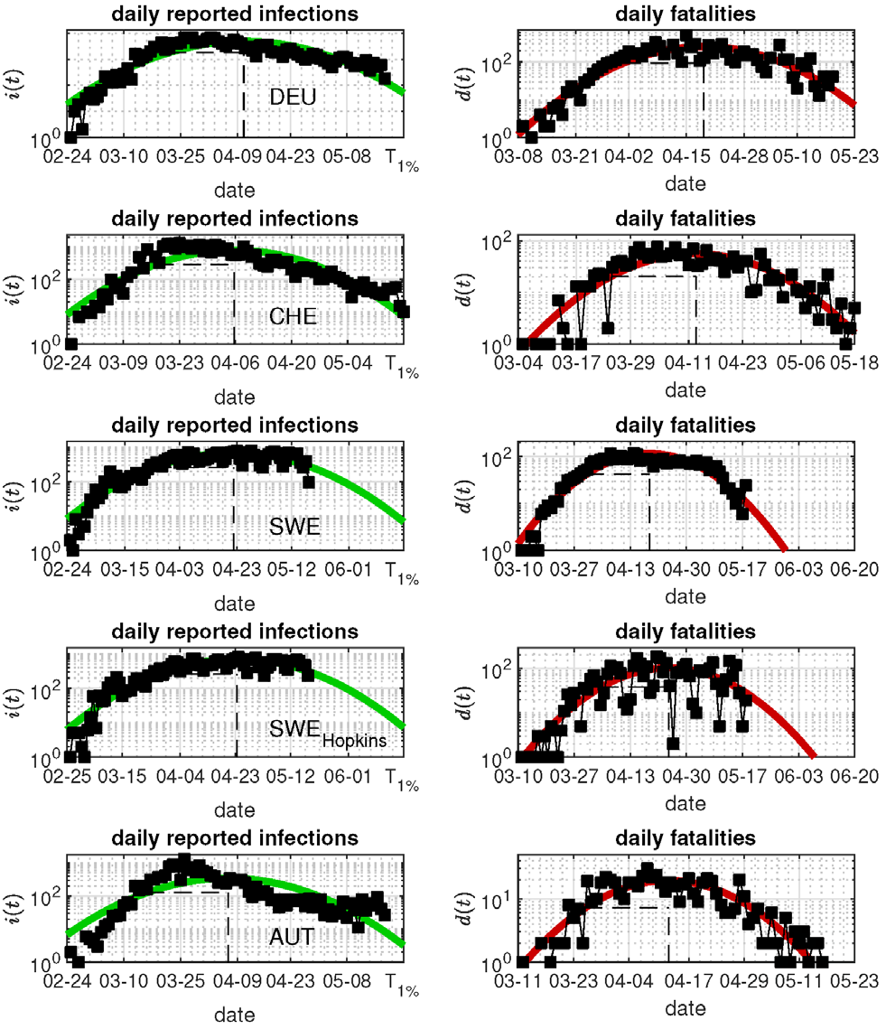
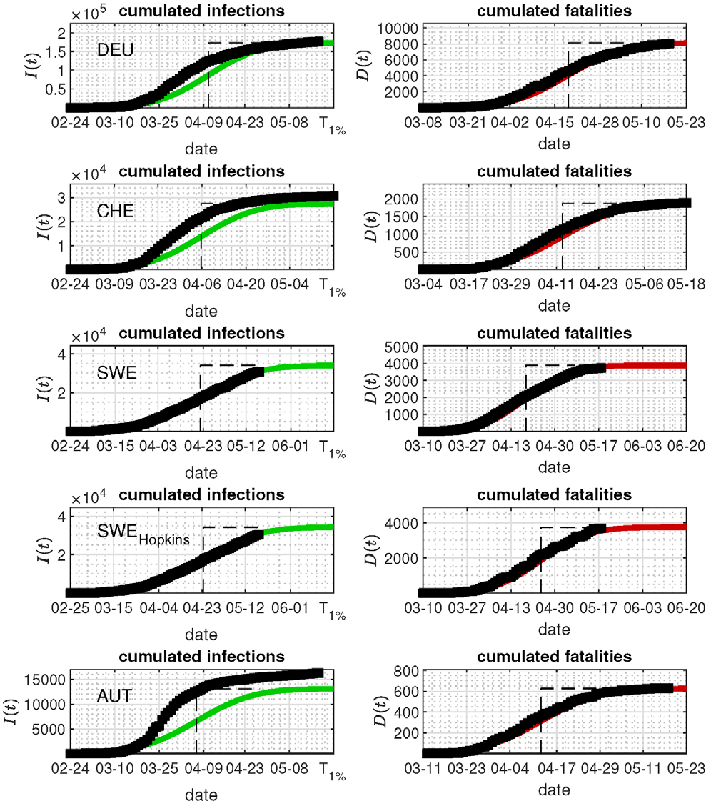
Figure 2: Cumulative number of reported infections (left) and cumulative number of deaths (right) in Germany (DEU), Switzerland (CHE), Sweden (SWE), and Austria (AUT) in comparison with the best fit from the GM. Fit from May 19, 2020. The dashed vertical lines indicate the peak times. As we know from Figure 1, cumulative reported infections must not be captured by the GM, as they do not coincide with the truly infected individuals.
Relationship between Parameters of the GM
We notice first that the reported Gaussian widths parameters wi for the infections and wd are of comparable and al- most equal value. The corresponding times of maximum are shifted to each other with td,max = ti,max + τ , where the delay peak time of deaths with respect to the peak time of infections τ ∈ [6, 8] days.
Dark Number of Infections
With the GM parameters at hand, the estimated total number of cases corresponding to the area under the curves shown in Figure 1, are available from equation (7). From the inferred values of D_tot and _I_tot we obtain an estimate of the unreported ”dark” number of infections via equations (8) and (9) with the following argument: Let γ = 0.5γ∗ be the fraction of seriously sick individuals in the hospital, estimated to α∗ percent of all infected people (typically α∗ = 1), who die from Covid-19. We use and carry on α∗ and γ∗ here and throughout this manuscript to understand how a departure of γ∗ and α∗ from unity would affect the conclusions. Both γ∗ and α∗ can be considered unity and erased from all equations, if the present estimates remain valid [31]. The fatality rate can be smaller: the recent Gangelt study [31] suggests γ = 0.37 (corresponding to γ∗ = 0.74) with a rather significant error. Dividing _D_tot by the fraction f of seriously sick out of all infected people, where _f = 0.01γα∗ = 5 10−3γ∗α∗, we can estimate the total true (reported plus unreported) number of infected individuals according to equation (8) as
200_D_ I γ α = (10)
true tot tot * * Consequently, the dark number of infections (9), i.e. the number of infected individuals unreported for each reported, is
200 1 d D N I γ α = − (11)
tot * * tot The last column of Table 1 lists the resulting dark numbers in the four countries.
Herd Immunity
After inserting the estimated number of _D_tot for a specific country we obtain the total true number of infected people, relevant to rate the degree of herd immunity or “indirect protection” [32], according to equation (8). In Germany with _D_tot/MP = 8150±2500 per million people (MP) from Tabele 1 we obtain ( ) true tot,Germany * *
1.6 0.5 I γ α ± =
million people, (12) which includes the dark number of infections. The corresponding values for the other countries are 0.37±0.08 (CHE), 0.76 ± 0.14 (SWE), 0.13 ± 0.04 (AUT) million people.
Breathing Apparati Capacity in Germany
With the estimated total death toll _D_tot/MP per million people (MP) we calculate the total number of seriously sick people from the true number of infected individuals Itrue by making use of the relationship (7) between daily and total number of cases. We thus infer for the maximum number of seriously sick individuals per day (NSSPs) and per million people
| 2D tot MP | |
|---|---|
| πw γ |
The resulting numerical values are available from Tabele 1 and discussed below.
Quarantine Factor
In the earlier analysis [28] the quarantine factor q≤1 had been introduced to account for the non-pharmaceutical interventions (NPIs), i.e. political actions and social measures in order to reduce the number of infections, such as quarantining of elder and infected people, social distancing actions, mask obligations as well as the closure of schools and daycare facilities. If none of these actions are applied then q = 1 and the canonical fraction 2/3~0.67 of the total population is infected. Scaling the total population in units of MP we then note that 0.67_q_ MP are infected during the whole duration of the first wave. With the already mentioned fatality rate 0.5γ∗ and the percentage α∗ = 1 of NSSPs the expected upper limit of the total number of fatalities per million people is given by tot,limit 5 * * * * 0.5 0.01 .6.7 10 3333 D q q MP γ α γ α = = (14) where [ ] 0,1 q∈ is the quarantine factor to be evaluated below using (14), and we are going to use γ∗= α∗= 1 as mentioned already
Discussion
Relationship between Parameters of the GM
The delay peak time of deaths with respect to the peak time of infections τ∈[6, 8] days is in agreement with earlier estimates [27]. An exception is the first dataset for Sweden, for which both peak times are identical within errors. A delay τ close to 7 days is perfectly compatible with the mean value of the gamma-shaped serial interval distribution in use to define and calculate reproduction factors [33, 34, 35, 36, 37].
Dark Number of Infections
The dark number of infections Nd we reported for selected countries in Table 1. For Germany we obtain Nd = 8.4 4.0. Hence, up to one of about 10 infected people had been recognized as being infected by testing. Despite the partially large 95-percent confidence errors also for other countries, which were however of similar magnitude when we performed the analysis one month ago, these determinations of the dark numbers in different countries by using the modeled infection and death rates is a strong advantage of the Gauss model. If this method is applied it serves as important benchmark to judge on the completeness of testing large portions of the population. For countries that cannot afford the laborious, time- consuming and costly testing our method still provides them with a reliable estimate of the fraction of infected persons.
Herd Immunity
The total true number of infected people, which we obtained by way of equation (8), allows us clues on the amount of herd immunity from the first wave. The estimate (12) implies that only 1.9 0.6 percent of the German population (P = 83 million people) will be infected in total by the first pandemic wave, leaving more than 98 percent of the German population to be potentially infected by the second and future pandemic waves. If these future waves infect a similar percentage of the population under the same strict social distancing measures, we expect more than 20 waves to occur over the next years until 2/3 of the total population in Germany are immunized, unless an efficient anti-Covid-19 vaccine is available soon. This is a frightening prospect, and optimized strategies for the man ageing of future pandemic waves have to be developed urgently. We address this further below more quantitatively.
Breathing Apparati Capacity in Germany
With the estimated total death toll in Germany of D_tot/ MP= (8150 ± 2500)/83 = 98 ± 30 per million people (MP) we calculate the total number of seriously sick individuals by dividing by the fatality rate γ = 0.5γ∗ to obtain (196 ± 60)/γ∗ per million people. According to the equation (7) with _wd = 18.0 ± 0.1 we then find for the maximum number of seriously sick individuals per day (NSSPs) per million people ( ) S
196 60 NSSP 6.1 1.9 MP d w γ π γ ± ± = = (15)
* * On the other hand in Germany currently there are approximately 40000 breathing apparati in total available, corresponding with P = 83 MP to 482/MP. With a typical breathing time of 10w∗ days or less (where in accord with our notation, w∗ is a number of order unity), German hospitals have the capacity of handling 48w∗ −1/MP NSSPs at the peak time of the first wave, which is more than a factor 7 greater than the maximum value (15). Fortunately, only about 19 percent [24] of the German breathing apparati capacity had to be used to treat the maximum number of NSSPs during the peak day of the first wave.
Quarantine Factor
By equating the expected limiting value (14) of total fatalities with the GM predictions for _D_tot for different countries we obtain an estimate of the corresponding values of the quarantine factor. For the standard values γ∗ = 1 and α∗ = 1 we obtain the quarantine factors given by Table 2. For Sweden we thus find a significantly higher value.
| Country | Code | P | Dtot/MP | q |
|---|---|---|---|---|
| Germany | DEU | 83 | 98 ± 30 | (2.9 ± 0.9)×10−2 |
| Switzerland | CHE | 8.5 | 200 ± 40 | (6.0 ± 1.2)×10−2 |
| Sweden | SWE | 10.5 | 370 ± 70 | (11.1 ± 2.1)×10−2 |
| Austria | AUT | 8.7 | 69 ± 23 | (2.1 ± 0.7)×10−2 |
Table 3: Quarantine factors q for countries considered in this work.
The influential Imperial College study [38] has listed the following five possible non-pharmaceutical interventions (NPIs) determining the quarantine factor: (1) CI: Case isolation in the home, (2) HQ: Voluntary home quarantine, (3) SDO: Social distancing of those over 70 years of age, (4) SD: Social distancing of entire population, and (5) PC: Closure of schools and universities. Based on the drastic measures taken in Germany and Switzerland we like to add as sixth NPI the closure of nonessential non-food shops and industry (CSI) imposed strictly in Austria, Germany and Switzerland [38].
These NPIs have been differently applied in the above 4 countries which have a comparable ethnic composition and standard of living: whereas Austria and Germany had been very strict, Switzerland didn’t apply SDO, SD, and PC strictly, Sweden has only applied CI, closure of universities and a mild form of SD. Therefore we are able to weight two combinations of the six NPIs actions with a quantitative number $r$, where
$$r_{\text{CI}+\text{SDO}+\text{SD}} \approx 10, \quad r_{\text{HQ}+\text{PC}+\text{CSI}} \approx 20,$$ (16)
The quarantine factor is then given approximately by the reciprocal sum
$$q \approx \frac{1}{\sum_i r_i}$$ (17)
While Austria and Germany have strictly applied all six NPIs, Switzerland has applied them in a less strict fashion, Sweden only applied three of them.
If hypothetically Germany, during the next waves, would only apply the mild NPIs Sweden has chosen for the first wave, the resulting quarantine factor would be $q_2 = 0.1$. With this value the expected total number of fatalities from the 2nd wave is
$$\frac{D_{\text{tot},2\text{nd}}}{MP} = 0.5\gamma_*0.01\alpha_*.6.7q_210^5 = 333\gamma_*\alpha_*$$ (18)
As in equation (15) we then find for the maximum number of seriously sick persons per day (NSSPs) per million people during the second wave
$$\frac{\text{NSSPs}}{\text{MP}} = \frac{333\gamma_*\alpha_*}{\sqrt{\pi w_d\gamma_*}} = 14.3\alpha_*$$ (19)
which German hospitals can handle even with the presently available capacity to treat up to $48w^{-1}/MP$ NSSPs. At unchanged $q$, the ratio NSSPs/MP is going to drop during subsequent waves, as the number of immune people will grow with each wave.
The limited breathing apparatus capacity at least in Germany is no good justification to apply the additional strict NPIs, i.e. voluntary home quarantine, closure of schools and universities as well as the closure of nonessential non-food shops and industry (CSI), also to the second and future waves.
**Summary and Conclusion**
Based on the lessons learned from the first wave of the Covid-19 pandemic disease and their analysis with the Gauss model we suggest the following recommendations for handling the 2nd and further waves.
The fraction of the total population $P$ that has developed antibodies during the first wave is given by $1/\sum_i r_i$. So for Germany with $P \approx 83$ million inhabitants, as noted, only approximately $1.9 \pm 0.6\%$ will have developed antibodies. In the light of this small percentage, or the small herd immunity, first there is no compelling reason to wait for the first wave to terminate completely. We could start continuing our daily lives at an- other level of social distancing immediately. Or as soon as sufficient amounts of masks will be available. Masks must not be perfect. Masks from linen that can be washed, and do not pollute our environment further, should be a preferred option. Any day ending the economical lockdown earlier is worth a thought: it would reduce the currently planned extremely high level of public indebtedness significantly, lower the risk of inflation, and save the public enormous amounts of financial resources that could be better used in improving the public health system to cope with the unavoidable 2nd and later pandemic waves.
Secondly, the 2nd and future waves could be handled with the mild NPIs that Sweden has so far applied during the first wave: case isolation in the home and a mild form of social distancing. Social distancing will be the main non-pharmaceutical intervention for the majority of the population. This will not seriously affect the daily lifes of most of the populations and avoid dramatic economical consequences. These mild NPIS should be simultaneously accompanied by the running analysis with the Gauss model that provides reliable predictions for several future weeks for the effectiveness of the taken measures, and if necessary allows implementing in due time stricter social interventions. The swedish approach with mild NPIs is not without risk: it definitely has led to a significantly higher death rate than in other neighboring countries. If no effective vaccination against Covid-19 is available in the next several years their higher herd immunity from the first wave might be an advantage in the long run. If an effective vaccination is available soon the swedish approach does not have to be copied by other countries.
Third, the strict and months-long lock-down seems to reflect the hope that the pandemic can be completely stopped. This appears very questionable. In view of the about 98% of the population for which the 2nd wave is basically identical with the 1st wave, and if we proceed with the current strategy, many complete lock-downs featuring unused capacities will follow. If such lock-downs are not planned, there is or was no reason to keep the present one for an extended period. A sufficient amount of social distancing can be applied immediately, also without masks and gloves. All it requires is inhabitants to overtake responsibility, and to change our daily lives.
As a final remark we mention that from the about 930000 people who died 2017 in Germany, about 344000 died from sometimes stress-related heart diseases (this annual number exceeds the total number of fatalities caused by Covid-19 without non-pharmaceutical interventions, as long as hospitals are not overloaded) about 25000 died in the 2018/2019 season from influenza [24]. The number of fatalities caused by car accidents decreased from about 20000 per annum in 1970 down to 3000 in 2019. On one hand a complete shutdown could therefore be considered to prevent fatalities in every year, on the other does it remains unclear yet, if there won’t be any socioeconomic or health- related issues that diminish the efforts.
References
-
Kermack WO, McKendrick AG (1991) Contributions to the mathematical theory of epidemics-I. Bull. Mathem Biol 53(1-2): 33-55.
-
Kermack WO, McKendrick AG (1932) Contributions to the mathematical theory of epidemics. II. -The problem of endemicity. Proc R Soc Lond 138(834): 55-83.
-
Kermack WO, McKendrick AG (1933) Contributions to the mathematical theory of epidemics-III.3-Further studies of the problem of endemicity. Proc R Soc Lond 141(843): 94-122.
-
Enserink M, Kupferschmidt K (2020) With covid-19, modeling takes on life and death importance. Science 367(6485): 1414-1415.
-
Barmparis GD, Tsironis GP (2020) Estimating the infection horizon of covid-19 in eight countries with a data-driven approach. Chaos, Solitons & Fractals 135: 109842.
-
Lixiang L, Yang Z, Dang Z, Meng C, Huang J, et al. (2020) Propagation analysis and prediction of the covid-19. Infect Disease Model 5: 282-292.
-
Ciufolini I, Paolozzi A (2020) Mathematical prediction of the time evolution of the covid-19 pandemic in italy by a gauss error function and monte carlo simulations. Eur Phys J Plus 135: 355.
-
Pham H (2020) On estimating the number of deaths related to covid-19. Mathematics 8(5): 655.
-
Cakir Z, Savas HB (2020) A mathematical modelling approach in the spread of the novel 2019 coronavirus sars-cov-2 (covid-19) pandemic. Electr J Gen Med 17(4): 205.
-
Alimadadi A, Aryal S, Manandhar I, Munroe PB, Joe B, et al. (2020) Artificial intelligence and machine learning to fight covid-19. Physiol. Genomics 52: 200-202.
-
Tarnok A (2020) Machine learning, covid-19 (2019- ncov), and multi-OMICS. Cytometry 97(3): 215-216.
-
Wynants L, Van Calster B, Bonten MMJ, Collins GS, Debray TPA, et al. (2020) Prediction models for diagnosis and prognosis of covid-19 infection: systematic review and critical appraisal. Brit Medic J 369: 1328.
-
Singh D, Kumar V, Vaishali, Kaur M (2020) Classification of covid-19 patients from chest CT images using multi- objective differential evolution-based convolutional neural networks. Eur J Clin Microbiol Infect Dis 39(7): 1379-1389.
-
Naude W (2020) Artificial intelligence vs covid-19: limitations, constraints and pit falls. AI Society 28: 1-5.
-
Kim S, Seo YB, Jung E (2020) Prediction of covid-19 transmission dynamics using a mathematical model considering behavior changes in Korea. Epidemiol Health 42: e2020026.
-
Zhu Y, Chen YQ (2020) On a statistical transmission model in analysis of the early phase of covid-19 outbreak. Stat Biosci 2: 1-17.
-
Bai ZH, Gong Y, Tian XD, Cao Y, Liu WJ, et al. (2020) The rapid assessment and early warning models for covid-19. Virol Sin 35(3): 272-279.
-
Wolfram C (2020) An agent-based model of covid-19. Complex Systems 29: 87-105.
-
(2020) Covid-19 forecasts from CDC.gov.
-
Sperrin M, Grant SW, Peek N (2020) Prediction models for diagnosis and prognosis in covid-19. Brit Medic J 369: m1464.
-
Kristiansen S, Burger EA, De Blasio BF (2020) Covid-19: Simulation models for epidemics. Tidsskriftet De Norske Laegeforening 140(6): 546-548.
-
Panovska Griffiths J (2020) Can mathematical modelling solve the cur- rent covid-19 crisis?. BMC Public Health 20(1).
-
Shrivastava SR, Shrivastava PS (2020) Resorting to mathematical modelling approach to contain the coronavirus disease 2019 (covid-19) outbreak. J Acute Disease 9(2): 49-50.
-
(2020) Database of the federal statistical office of Germany, Statistisches Bundesamt destatis.
-
(2020) Official statistics at arcgis, public health agency of Sweden.
-
Kröger M (2020) Covid-19 real time statistics & extrapolation using the gauss model. GM Website.
-
Schüttler J, Schlickeiser R, Schlickeiser F (2020) Covid-19 predictions using a gauss model, based on data from April 2. Physics 2: 197-212.
-
Schlickeiser R, Schlickeiser F (2020) A gaussian model for the time development of the sars-cov-2 corona pandemic disease. Predictions for Germany made on March 30, 2020. Physics 2: 164-170.
-
Farr W (1840) Causes of death in England and wales. Annual Report of the Registrar General of Births, Deaths and Marriages in England 2: 69-98.
-
(2020) Json time-series of coronavirus cases (confirmed, deaths and re-covered) per country-updated daily. Github contributors as of April 2.
-
Streek H, Hartmann G, Exner M, Schmidt M (2020) Preliminary results and conclusions of the covid-19 case cluster study (Gangelt Municipality).
-
Fine P, Eames K, Heymann DL (2011) Herd immunity: A rough guide. Clin Infect Diseases 52(7): 911-916.
-
Milligan GN, Barrett ADT (2015) Vaccinology: an Essential Guide. Wiley, pp: 200.
-
Fraser C, Donnelly CA, Cauchemez S, Hanage WP, Van Kerkhove MD, et al. (2009) Pandemic potential of a strain of influenza A (H1N1): Early findings. Science 324(5934): 1557-156.
-
Flaxman S, Mishra S, Gandy A , Unwin HJT, Coupland H, et al. (2020) Estimating the number of infections and the impact of no pharmaceutical interventions on COVID-19 in 11 European countries: Technical Description Update. Cornell University.
-
Scirea J, Nadeaua VT, Brupbacher C, Fuchs S, JSommer J, et al. (2020) Re-productive number of the covid-19 epidemic in Switzerland with a focus on the cantons of basel-stadt and basel-landschaft. Swiss Medical Weekly 150: 20271.
-
Kröger M, Schlickeiser R (2020) Gaussian doubling times and re- production factors of the covid-19 pandemic disease. Frontiers in Physics 8: 276.
-
Ferguson N, Laydon D, Nedjati Gilani G (2020) Impact of non- pharmaceutical interventions (NPIs) to reduce covid-19 mortality and healthcare demand. Imperial College London, pp: 1-20.
-
(2020) OECS data, organization for economic co- operation and development (OECD).
- Epidemiological Surveillance and Rumors on Social Media
- Awareness and Treatment of Uncontrolled Hypertension in US Overweight/Obese Youths Aged 16–24 Years, NHANES 2021–2023
- Strengthening EPI Through Parental Engagement: Lessons from Dhaka Slums for IA-2030
- Mothers Knowledge of the Prevalence, Causes, Effects, Prevention and Control of Diarrhoea among Children in Ife East Local Government Area, Ile Ife, Osun State, Nigeria
- Covid-19 Reinfections Case Series from October 2023 to October 2024 in A General Medicine Office in Toledo (Spain)
- Water Contact! One Risk Too Many: Risk Factors Associated with Schistosoma haematobium infection in Osun State, Nigeria