Regional Method for Israel COVID-19 Forecast

Introduction

In the contemporary research community, the statistical aspects of COVID-19 and other recent epidemics of a similar nature were receiving considerable attention [1]. In general, using traditional theoretical statistical methods to determine outbreak probabilities and realistic health system reliability factors under actual epidemic conditions is quite difficult [1, 2, 3]. The only observation figures for COVID-19, however, are constrained to the first of 2020. Israel was obviously selected because to its COVID-19 origin, substantial health monitoring, and available internet research [4, 5]. This study relied on the quasi-stationarity assumption; the underlying epidemiological process was assumed, although seasonally varying but still statistically representative during two 2020-2022 years of continuous observation. The underlying trend must be addressed in the longer time horizon. Note that although analysed data set is quite limited both in time (only two years) as well as in space (only state of Israel), the proposed methodology has already been well validated in other studies by authors Gaidai O, et al. [6, 7, 8, 9, 10, 11, 12, 13, 14, 15, 16, 17, 18, 19].

Methods

A suitably enough period of time has been used to assess the MDOF health system response vector process ( ) ( ) ( ) ( ) ( ) , , , t X t Y t Z t = … ( ) 0,T . Unidimensional global maxima over the full period ( ) 0,T are ( ) max

0max T t T X X t ≤≤ = , ( ) max

0max T t T Y Y t ≤≤ = ,

( ) max

0max , T t T Z Z t ≤≤ = … see Fig. 2. One generally implies a big value of with regard to the dynamic system auto-correlation time when they refer to a suitably lengthy duration. Let

1, , X N X X … represent subsequent local maxima of the process ( ) X t at discrete temporally increasing time instants X X N t t <…< in time( ) 0,T . For other MDOF response

1 X components, such as ( ) ( ) , , Y t Z t etc, the analogous definition is as follows: 1 , , ; Y N Y Y … 1, , Z N Z Z … and so on.

For the sake of simplicity, it is assumed that all of ( ) t R

components and their maxima are positive. The goal is to calculate the likelihood of a system failing, specifically the likelihood of exceeding, accurately max max max 1 Prob( ) T X T Y T Z P X Y Z η η η − = > ∪ > ∪ > ∪… (1) W h e r e ( ) ( ) η η η … , , , max max max max max max , , , 0, 0, 0, , , , , X Y Z … … = … … Y z T T T T T T T N N X Y Z P p X Y Z dX dY dZ max max max ( ) is the likelihood that critical values of the response components , , ,… will not be exceeded; stands for the logical unity operation «or»; and max max max , , , T T T X Y Z p … is the joint probability density of the global maxima throughout the whole time( ) 0,T . Due to its large dimensionality and the limits of the provided data set, it is not practical to directly estimate the latter joint probability distribution. More specifically, the health system is considered to have failed instantly when either ( ) X t exceeds X η , ( ) Y t exceeds Y η , ( ) Z t exceeds , and so on. For each unidimensional response component of R(t), fixed failure levels X η , Y η , Z η ,...

are, of course, unique ( )t R . max max max { ; 1, , } X N j X T X X j N X = = … = , max max max { ; 1, , } Y N j Y T Y Y j N Y = = … = , max max max { ; 1, , } z N j Z T Z Z j N Z = = … = , and so forth. Time instants at local maxima X X Y Y Z Z N N N t t t t t t   <…< <…< <…<   are

1 1 1 ; ; X Y Z

combined into a single time vector, 1 N t t ≤…≤ , in monotonously non-decreasing order. Keep in mind that X Y Z N N N N t t t t = … , X Y Z N N N N = + + +… .

max { , , , } X Y Z

In this instance, the local maxima of one of the MDOF structural response components, such as ( ) X t or ( ) Y t , or ( ) Z t , and so on, are represented by . This means that, given a R(t) time record, all that is required to record a component’s MDOF limit vector ( ) , , ,... X Y Z η η η exceedance in any of its components is to continuously and simultaneously screen for local maxima in the unidimensional response component. Following the merged time vector 1 N t t ≤…≤ , local unidimensional response component maxima are combined into a single temporal non-decreasing vector ( ) 1 2 , , , N R R R R = … ρ . In other words, each local maxima Rj corresponds to an actual encountered local maxima for either ( ) X t or ( ) Y t , or ( ) Z t , and so on. The unified limit vector ( ) 1, , N η η … is then introduced, and each component j η is either an X η , Y η or Z η component, depending on which of ( ) X t or ( ) Y t , or ( ) Z t , etc, corresponds to the running index ‘s current local maxima. The new MDOF limit vector ( ) , , ,... X Y z λ λ λ η η η with . X X λ η λ η ≡ , . X X λ η λ η ≡ , . z Z λ η λ η ≡ ,... is introduced, along with the caling parameter0 1 λ < ≤ , to artificially simultaneously decrease limit values for all response components. Each component of the unified limit vector ( ) 1 , , N λ λ η η … is named j λ η and is either X λ η , Y λ η or z λ η , and so on. The latter defines probability ( ) P λ automatically as a function of λ ; take note that ( )1 P P ≡ from Eq. (1). Non- exceedance probability ( ) P λ will be now estimated as follows ( ) { } 1 1 Prob , , N N P R R λ λ λ η η = ≤ … ≤ { } 1 1 1 1 1 1 1 1 Prob{ | , , } Prob , , N N N N N N R R R R R λ λ λ λ λ η η η η η − − − − = ≤ ≤ … ≤ ⋅ ≤ … ≤ N ( ) 1 1 1 1 1 1 2 Prob{ | , , } Prob j j j j j R R R R λ λ λ λ η η η η − − = = ≤ ≤ … ≤ ⋅ ≤ ∏ (2) In practice, dependence between neighbouring jR is not always negligible; thus, the following one-step (will be called here conditioning level 1 k = ) memory approximation being introduced

1 1 1 1 1 1 Prob{ | , , } Prob{ | } j j j j j j j j R R R R R λ λ λ λ λ η η η η η − − − − ≤ ≤ … ≤ ≈ ≤ ≤ (3) for 2 j N ≤ ≤ (conditioning level ). The approximation introduced by Eq. (3) will be further expressed as

1 1 1 1 1 1 2 2 Prob{ | , , } Prob{ | , } j j j j j j j j j j R R R R R R λ λ λ λ λ λ η η η η η η − − − − − − ≤ ≤ … ≤ ≈ ≤ ≤ ≤ (4) where 3 j N ≤ ≤ (will be called conditioning level 3 k = ), and so on. Subsequent improvements to the statistical independence assumption are presented in Eq. (4). This study makes the assumption that the entire health system, including all of its dimensions, is stationary. As a result, the constructed process ( )t R is also assumed to be stationary. Since original MDOF process ( )t R is stationary because it is assumed to be ergodic, the probability will be independent of j but solely dependent on conditioning level k for j k ≥ . So, it is possible to approximate non-exceedance probability using the average conditional exceedance rate method.

( ) ( ) exp ( . ) , 1. k k P N p k λ λ ≈ − ≥ (5)

It should be noted that Eq. (5) deduces from Eq. (1) by ignoring ( ) 1 1 Prob 1 R λ η ≤ ≈ and assuming N k  because the probability of a design failing must be extremely low. The well-known mean up-crossing rate equation for the probability of exceeding is comparable to Eq. (5) [20]. There is evident convergence with respect to the conditioning parameter k ( ) ( ) ( ) lim 1 ; lim k k k k P P p p λ λ →∞ →∞ = = (6) Note that Eq. (5) for 1 k = turns into a known non- exceedance probability expression for the mean up-crossing rate function ( ) ( ) ( ) ( ) 0 exp ( ); , RR P T p d λ ν λ ν λ ζ λ ζ ζ ∞ + + ≈ − = ∫  (7) Where ( ) ν λ + stands for the mean up-crossing rate of the response level for the non-dimensional vector ( ) R t above that was constructed from scaled MDOF system response   …     X Y Z η η η , , , . Rice’s formula, which is given in Eq. (7), X Y Z yields the mean up-crossing rate, where is the joint probability density for( ) , R R , where is the time derivative ( ) ' R t . The Poisson assumption, which is the basis for Eq.

(7), states that up-crossing events with high λ levels (in the current study, it is 1 λ ≥) can be assumed to be independent. The stationarity assumption was applied in the examples above. The nonstationary case, however, can also be handled by the suggested methodology. Each short-term seasonal state has a probability of m q in the nonstationary case’s scattered diagram of 1,.., m M = seasonal epidemic M = = ∑ . Next, let one introduce m m q

1 1 conditions, meaning that the long-term equation M

( ) ( ) = ≡∑ (8)

k k m m p p m q λ λ

1 , With ( ) , kp m λ being same function as in Eq. (6), corresponding to a specific short-term seasonal epidemic state with the number . The ( ) kp λ functions mentioned above are frequently regular in the tail, especially for values of approaching and exceeding 1. More specifically, for 0 λ λ ≥ , the distribution tail behaves as ( ) { } exp c a b d λ − + + , where a, b, c, d are appropriately fitted constants for an appropriate tail cut-on 0 λ value. Therefore, one can write ( ) ( ) { } 0 exp , kc k k k k p a b d λ λ λ λ ≈ − + + ≥ (9) Next, nearly perfectly linear tail behavior is seen by plotting ( ) ( ) { } ln ln k k p d λ − versus ( ) ln k k a b λ + .

Sequential quadratic programming (SQP), a tool included in the NAG Numerical Library, can also be used to find the parameters , , , , k k k k k a b c p q ideal values [8, 9, 10, 11, 12, 13, 14, 15, 16, 17, 18, 19].

Results

In both epidemiology and mathematical biology, the prediction of influenza-like epidemics has long been the main focus. The website that presents COVID-19 data from Israel is where the statistical information in this section is taken from [4]. The website provides numbers of newly diagnosed and death cases every day in Israel from 22 January 2020 to 6 April 2022. In order to illustrate a two-dimensional (2D) dynamic health system, patient numbers from two distinct Israel health recorded categories—daily recorded patients and deaths, respectively-were selected as components. In order to unify both two measured time series X, Y the following scaling was performed X Y X Y η η → → (10) , X Y

Making both two responses non-dimensional and having the same failure limit equal to 1. In the current study, failure limits, or alternatively epidemic thresholds, were set at the observed two-year maxima, twice increased, for each category of the health system. Then, all local maxima from both measured time series were combined into a single time series while maintaining their temporal non-decreasing order: { } { } ( ) 1 1 max , , ,max , N N R X Y X Y = … ρ with the entire vector being sorted in temporally non-decreasing order of these local maxima’s occurrence.

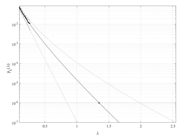
Figure 1 presents 100-years return level extrapolation in accordance with Eq. (9) towards epidemic outbreak with

100-year return period. This extrapolation is shown by the horizontal dotted line, and a cut-off value of was used to further extrapolate it. According to Eq. (10), dotted lines represent the extrapolated 95% confidence interval (CI). The goal failure probability 1 P − from Eq. (5) is directly connected to ( ) p λ according to that equation Eq.(1). In Figure 1, the star symbolizes the expected non-dimensional λ level, which denotes the likelihood that an epidemic would break out at any given level of the Israeli health system in the years to come. For the method validation, the asymptotic Gumbel generalized extreme value (GEV) distribution was applied, namely extrapolation was done on Gumbel probability plot, prediction was found located within 95% CI, depicted in Figure 1.

Click to enlarge

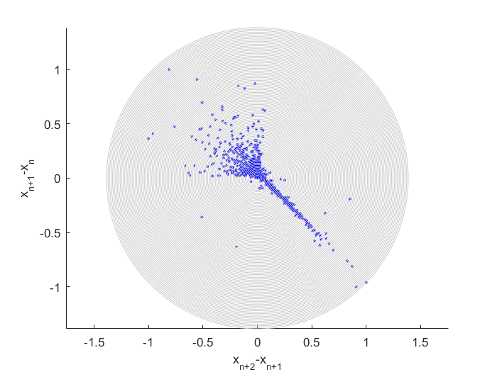
The Poincare plot is where the second-order difference plot (SODP) got its start. Time series data from SODP can be used to observe the statistical situation of consecutive differences.

Figure 2 presents SODP plot, this type of plot can also be used to identify data patterns and compare them to other data sets, such as when using an artificial intelligence (AI) recognition method based on entropy [21]. Figure 2 indicates unnatural correlation pattern - the reason for that is presence of the straight diagonal line pattern Figure 2, not present on other national COVID-19 data SODP plots, for example Norway. SODP plot straight diagonal line means that large portion of the data consecutive differences 2 1 n n x x + + − being almost equal to 1 n n x x + − , which is un-physical and at least raises suspicions, at most may indicate the data rigging. Keep in mind that while this paper presents MDOF and a sub-asymptotic method, extreme value theory (EVT) is asymptotic and 1DOF. Despite its apparent simplicity, the current work presents a unique multidimensional modeling technique and a methodological route to apply epidemic forecasting while it is still in progress.

Click to enlarge

Discussion

The disadvantage of coping effectively with systems with high dimensionality and cross-correlation between various systems responses is not present in traditional health systems dependability approaches dealing with observed time series. The capacity to examine the dependability of high dimensional non-linear dynamic systems is the main benefit of the approach that has been developed. Despite its apparent simplicity, the current work presents a unique multidimensional modeling technique and a methodological route to apply epidemic forecasting while it is still in progress. This study looked at recently reported COVID-19 patient and death figures from Israel, which is an illustration of a two-dimensional (2D) phenomenon that was seen in 2020– 2022. It should be noted that the provided strategy works effectively for more than simply two dimensional levels. As a result, the recommended technique may be useful for a range of dependability investigations on non-linear dynamic health systems.

Acknowledgements

The authors declare no conflict of interest. No funding was received. All authors contributed equally. The datasets analysed during the current study are available online.

Conflict of Interest

There are no conflicts to declare.