Application of Time Series Analyses in Forensic Accounting
This paper addresses how time series analyses can be used in forensic accounting by presenting three time series models and testing their relevance to forensic accounting practices. The ever-increasing business complexity and technological advances necessitate technological modernization in forensic accounting processes and the use of digital forensics. Time series analyses have been extensively used in areas such as sociology and marketing but not in forensic accounting. Previously undisclosed information is now available and can be used in forensic accounting services that extend beyond traditional forensic accounting. Time series models can be used to search millions of transactions to detect spot patterns and anomalies or irregularities. Examples are provided showing practical uses of time series models to aid in identifying fraud and non-fraud anomalies and red flags with considerably less resources. This study provides policy, educational, research and practical implications for forensic accounting.
Introduction
The existence and persistence of fraud can be detrimental to the quality of financial and non-financial information and forensic accountants can play an important role in preventing and detecting fraud. Forensic accountants should possess technical, analytical, and soft skills in effectively performing fraud investigation, litigation consulting, expert witnessing, and valuation services. We examine the relevance and use of time series analyses in forensic accounting by presenting time series models and providing three examples of how time series models can be efficiently and effectively applied in forensic accounting. The accounting literature addresses the application of time series analyses in accounting in an isolated fashion as reviewed in Section II [1]. A time series is a sequence of points, generally, over a period of equal time intervals (e.g., daily, weekly, monthly, and annually). Examples of time series are the daily closing value of the Dow Jones Industrial average, daily foreign exchange rates, and the number of students enrolled per semester [2, 3, 4, 5]. The application of time series models to forensic accounting is currently at a very early stage.
The increasing complexity of business, risk management, corporate governance, globalization, and the increasing demand for forensic accounting services reveal the need for the use of technology to modernize forensic accounting processes and the use of digital forensics. Digital forensics is a digital data analytics technique used in assessing evidence in online computer networks including computer forensics and network forensics [6]. Time series analyses have been extensively used in areas such as marketing and sociology but not in forensic accounting. Information that was not previously publicly disclosed is now available and can be used by forensic accountants in performing fraud investigation, litigation consulting, valuation, and expert witnessing services. Through the use of time series models, a great number of transactions can be searched to find existing patterns and detect anomalies or irregularities. Furthermore, the advances in digital forensics enable forensic accountants to employ time series analyses in an online and digital environment. We should note that time series analysis has some similarities with data mining; however, in data mining, researchers automatically search large piles of data from different angles or dimensions to discover trends or patterns in data, while in time series analysis, researchers focus on only one aspect of data to determine, trend, seasonal fluctuations, and irregularities [7].
Big data as well as greater access to detailed industry information, business, and media along with digital forensics help forensic accountants to better perform their forensic accounting services. Contrary to traditional financial transactions and report, more information is now available from social media such as e-mails, texts, and voices. In short, the availability of information now extends far beyond traditional risk assessment and fraud investigation. It should be noted that new and extended information as well as audit analytics bring the new challenges with them, challenges such as the availability of relevant data and experts to process and analyze the data and thus time series models can maximize the utilization of data. The main objective of this paper is to show how time series models can be used by forensic accountants and their organizations in performing forensic accounting services, detecting and preventing fraud, and performing non-fraud forensic accounting services. Forensic accountants can use time series analyses to identify red flags and accounting anomalies with spending considerably cost and time. Forensic accountants can use our suggested time series models to improve the quality of their forensic accounting services. Our models can be used in future research to advance empirical studies regarding forensic accounting and auditing. Accounting departments and business schools in general can also integrate time series analyses in their curricula to better educate future forensic accountants and business leaders.
The remainder of this paper is organized as follows: Section II explores prior time series studies relevant to accounting. Section III presents time series models and practical examples. Section IV provides comments and policy, practical, educational, and research implications of our study. The final section, Section V, presents concluding remarks.
Literature Review
Prior research finds that over 20 percent of firms intentionally misrepresent their earnings, about 20 percent of firms disclose early signals to investors regarding their material internal control weaknesses, and the existing financial and auditing systems provide inadequate incentives and accountability for management and auditors to protect investors from receiving misleading financial information [8]. According to the Association of Certified Fraud Examiners, ACFE business organizations every year lose about 5 percent of their revenues to fraud [9]. This loss can exceed $3.5 trillion. Prior studies show that fraud is detrimental to the quality of financial information and forensic accountants can play an important role in preventing and detecting fraud.
The literature reviewed in this section demonstrates that the use of time series models is in a preliminary stage in accounting and auditing as explained below. For
example, Welch explains the conceptual relationship between two models of asset pricing, namely Fama- French time series regressions and Fama-Macbeth cross sectional regressions and concludes that there is a close relationship between Fama-Mcbeth slopes and time series intercepts of Fama-French when all asset pricing restrictions are present [10, 11]. Moskowitz, et al. document important time-series moments in equity index, commodity, currency, and bond futures for 58 selected liquid instruments and show the significant momentum difference between the time-series momentum effect and the cross-sectional momentum effect even though these two are statistically correlated [3].
Zakamulin examines four benchmark indices and concludes that a detailed study of actual performance outperforms the commonly used market timing strategies [4]. Thus, investors should take into account the fact that market timing strategy probably underperforms a passive market strategy over a medium run period. Dudler, et al. introduce the risk-adjusted time series momentum (RAMOM) strategy that is calculated based on the averaging of returns of past and futures that are adjusted by the volatility of these returns, claiming that their strategy is very relevant and can be used for risk management [12].
Krahel and Titera state that accounting and business practices have moved to the use of Big Data and data analytics while the accounting and auditing standards have not changed from traditional focus on sampling practices to more sophisticated data analytics [13]. In this regard, Amir, et al. posit that disaggregation and broader disclosure of information help external users to better detect manipulation of financial statements and that time series data, together with newly developed sophisticated software as well as exponentially increasing power of computer hardware, help to better estimate future events [14]. Yoon, et al. argue that time series data should be used as complementary evidence in auditing for consideration of sufficiency, reliability, and relevance [15]. Consequently, time series data provides auditors with a variety of financial and non-financial information [16].
Baltas and Kosowski examine the effects of time-series momentum strategies on turnover and performance of their selected asset prices from 1974 to 2013 and conclude that more efficient models that consider the volatility in stock prices can significantly reduce the related portfolio turnover and, as a result, rebalance costs [5]. Gow, et al. evaluate methods used in accounting and auditing studies to correct the cross-sectional and time- series dependence and argue that most studies in accounting are cross-sectional and are serially correlated; most methods used are not correcting for this serial correlation [17]. Based on the examination of a total of 121 research studies that apply cross-sectional and time- series data in their regression analyses. Gow, et al. conclude that the majority of test results reported for accounting models are not specified correctly because they Ordinary Least Squares (OLS) [17]. Gow, et al. suggest the use of Feasible Generalized Least Squares (FGLS) in business research [17, 18, 19, 20].
Taken together, prior research has extensively focused on the time-series momentum and on the methods used by researchers to make adjustments for serial correlation with less attention to the implications of time series in accounting and auditing. In this paper we contribute to the literature by providing practical examples to show how time series models can be used in forensic accounting.
Time Series Model
Yule introduces autoregressive techniques during 1920s [21, 22, 23]. Before introducing autoregressive concepts, time series analysis was limited to drawing a simple estimation from a mass of data. Yule uses autoregressive techniques together with a linear regression model to predict sunspots [23]. Yule’s model has been extensively used in different fields such as marketing for forecasting future sales.
Initially, time series were used for forecasting and for this purpose time series are decomposed into four components: (1) time trend component, (2) seasonal component, (3) cyclical component, and (4) irregular component [7]. The long-term behavior of the series is captured by the time trend component, the intra year fluctuations that usually do not change from one year to another year with respect to magnitude, direction, and timing, the seasonal component, and the regular periodic changes that are captured by the cyclical component. Finally, the irregular component is represented by the stochastic or unknown component of the series.
Enders, et al. posits that the theory of difference equation is the foundation of the time series models [7]. That is, the econometrics of time series is dealt with the analyses of difference equations with the unknown (stochastic) component. As previously mentioned, time series analysis was initially used for forecasting or finding the time path of a variable. Finding the time path of a variable allows researchers to predict the future by examining the past behavior of a variable. The increasing demand for stochastic difference equations has highlighted the importance of the new role for time series econometrics. Time series models can be applied to different purposes such as interpretation of economic data, developing hypotheses, as well as for hypothesis testing [1]. In other words, the new role of econometricians is to develop new and appropriate time series models that can be utilized for data collections and interpretations, testing hypotheses, and forecasting.
Econometricians use time series models in many different fields and industries for preparing data, developing the best fitting curves, as well as queries and aggregation over a long-time period, and forecasting. Time series are used in many fields such as finance for predicting future stock prices by testing economics models (e.g., random walk, random walk with drift, and white noise). Time series analyses are extensively applied in many different industries (e.g., medical science, engineering, and medicine). In short, the initial application of time series analyses was for forecasting. For this purpose, econometricians have developed methods to break down a time series into: trend, cyclical, seasonal, and irregular components. The long-term behavior is shown by the trend component, the periodic component is shown by the cyclical component, and the random (stochastic) component is shown by the irregular component.
Time series analysis can be used as a powerful tool in continuous auditing. For example, Alles, et al. develop a continuous auditing system by taking three steps: (1) the first step is automatic verification of transactions, (2) the second step is developing a benchmark, and (3) the third step is applying the bench mark to each transaction to detect anomalies [24]. Vasarhelyi, et al. posit that the new audit method is expanding to include highly automated processes that are highly integrated and include components such as: control tags, automatic confirmations, continuous equations, and time series and cross-sectional analyses [25]. Alles, et al. discuss the efficiency and economics of continuous auditing and suggest that continuous auditing requires new infrastructure to enhance its efficiency [26].
As we mentioned above, accountants have not adequately and properly utilized time series analysis in practice and research even though there are many opportunities in which time series models can be applied properly. The main purpose of this paper is to show that, like other disciplines such as, medicine, finance, engineering, and medical science, time series models have many implications in accounting. Even many applications of time series in accounting can be listed, in this paper we provide three examples that show how time series models can be used in forensic accounting. We expect this paper can create an incentive for further research in forensic accounting.
Application of Time Series in Forensic Accounting
This section presents three examples of the application of time series in forensic accounting by using the data of three public companies that had exposure to fraudulent activities. We show how, by using appropriate time series models, the fraud exposure could have been caught and prevented in a timely manner. We posit that the historical data can be used to develop models that capture the behavior of data such as revenues, expenses, and net income, and then these models can be used to predict future revenues, expenses, and net income. These predictions can be compared with their related actual amounts to detect any deviation from the predicted amounts. To demonstrate these comparisons, we have developed three time series models for American International Group, Wells Fargo and Company, and West Management, respectively.
Modeling Quarterly Net Income of American International Group (AIG)
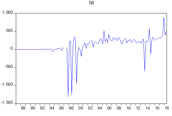
Quarterly net income of American International Group (AIG) for periods from the first quarter of 1979 to the first quarter of 2018 is collected from the Research Insights (Compustat) data base. Figure 1 shows the plot of quarterly net income of AIG for each quarter from the first quarter of 1979 to the first quarter of 2018.
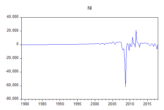
(Net Income (NI) presented in millions of dollars) Figure 1: Plot of Quarterly Net Income of AIG (1979 - 2018).
Different time series models are examined, and different model selection criteria are compared. Our comparisons indicate that the first order autoregressive model, AR (1) best fits our observed data. Results of running AR (1) model are shown in Table 1:
𝑥𝑡= 𝛽0 + 𝛽1𝑥𝑡−1 …… (1) Where: 𝑥𝑡 : net income of AIG in quarter t 𝑥𝑡−1 : net income of AIG in quarter t - 1 Table 1 summarizes the regression outputs of Model 1, which includes data from the first quarter of 1979 to first quarter of 2018. Table 2 presents Autocorrelation (AC), Variable Coefficient Std. Error t-Statistic Prob. C 219.9989 1256.007 0.175157 0.8612 AR(1) 0.379661 0.028369 13.38309 0 SIGMASQ 30537367 925243.1 33.0047 0 R-squared 0.145961 Mean dependent var 217.8376 Adjusted R-squared 0.134869 S.D. dependent var 5998.8 S.E. of regression 5579.628 Akaike info criterion 20.11155 Sum squared resid 4.79E+09 Schwarz criterion 20.16995 Log likelihood -1575.756 Hannan-Quinn criter. 20.13526 F-statistic 13.15978 Durbin-Watson stat 1.977714 Prob(F-statistic) 0.000005
| AC | PAC | Q-Stat | Prob |
Table 1: Summary of Regression Output of Model 1.
Partial Auto Correlation (PAC), and Q-Stat as well as their significance. As shown in Table 1, the p-value (Prob.) of the coefficient of first lag of net income as well as the p- value of the coefficient of the variable that controls for serial correlation is close to zero, indicating that these two coefficients are significantly different from zero. Furthermore, the power of the test, represented by an adjusted R-Squared of 0.13, is reasonable, given the low number of independent variables included in the model. In addition, all model selection criteria such as Akaike Information Criterion, Schwarz Criterion, and Hannan- Quin Criterion are smaller than those for its competing models.
| AC | PAC | Q-Stat | Prob | |
| 1 | 0.382 | 0.382 | 23.355 | 0 |
| 2 | 0.129 | -0.02 | 26.047 | 0 |
| 3 | 0.137 | 0.111 | 29.1 | 0 |
| 4 | 0.183 | 0.112 | 34.543 | 0 |
| 5 | -0.001 | -0.138 | 34.543 | 0 |
| 6 | -0.025 | 0.009 | 34.645 | 0 |
| 7 | 0.017 | 0.01 | 34.692 | 0 |
| 8 | -0.17 | -0.237 | 39.554 | 0 |
| 9 | -0.098 | 0.094 | 41.171 | 0 |
| 10 | -0.049 | -0.035 | 41.583 | 0 |
| 11 | -0.023 | 0.008 | 41.673 | 0 |
| 12 | -0.229 | -0.188 | 50.728 | 0 |
| 13 | -0.152 | -0.016 | 54.735 | 0 |
| 14 | -0.112 | -0.066 | 56.935 | 0 |
| 15 | -0.1 | -0.005 | 58.711 | 0 |
| 16 | -0.016 | 0.09 | 58.754 | 0 |
| 17 | -0.034 | -0.073 | 58.959 | 0 |
| 18 | -0.062 | -0.044 | 59.652 | 0 |
| 19 | -0.048 | 0.036 | 60.073 | 0 |
| 20 | -0.044 | -0.172 | 60.432 | 0 |
Table 2: AC, PAC, Q-Stat, and Significance for AIG.
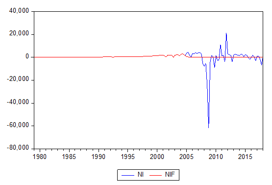
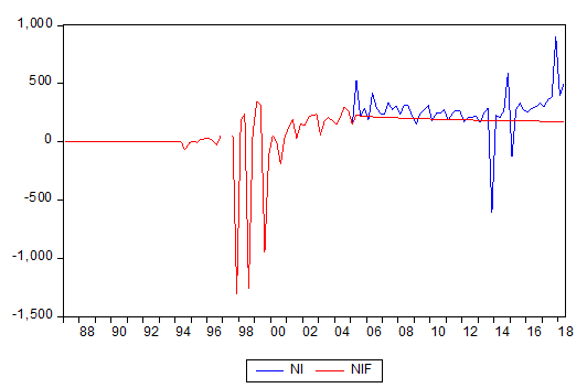
Using an AR (1) model, quarterly data from first quarter of 1979 up to the first quarter of 2005 are used to estimate net income of AIG from the second quarter of 2005 to the first quarter of 2018. As the following graph shows, the unusual deviation of actual net income from the forecasted net income could have been used as red flags, requiring more scrutiny and investigation as well as fraud prevention.
Modeling Quarterly Net Income of Wells Fargo and Company (WFC)
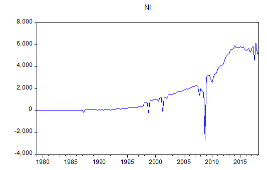
Data: Quarterly net income of Wells Fargo and Company (WFC) for periods from the first quarter of 1979 to the second quarter of 2018 is collected from the Research Insights (Compustat) data base. Figure 3 shows the plot of quarterly net income of WFG for each quarter from the first quarter of 1979 to the second quarter of 2018.
Variable Coefficient Std. Error t-Statistic Prob. C 1942.245 2039.63 0.952254 0.3425 AR(1) 1.90446 0.154012 12.36568 0 AR(2) -0.906054 0.153629 -5.897664 0 MA(1) -1.615648 0.146492 -11.02892 0 MA(2) 0.684316 0.098658 6.936266 0 SIGMASQ 284509.8 8582.424 33.15029 0 R-squared 0.929199 Mean dependent var 1565.253 Adjusted R-squared 0.92687 S.D. dependent var 2010.974 S.E. of regression 543.8203 Akaike info criterion 15.49529 Sum squared resid 44952556 Schwarz criterion 15.61159 Log likelihood -1218.128 Hannan-Quinn criter. 15.54253 F-statistic 398.9703 Durbin-Watson stat 1.957743 Prob(F-statistic) 0
- Dependent Variable: $y_t$
Table 3: Summary of Regression Output of Model 2.
Different time series models are examined and different model selection criteria are compared. Our comparisons indicate that the second order autoregressive together with second order moving average model, ARMA (2,2) best fits our observed data. Results of running ARMA (2,2) model are shown in Table 4:
𝑦𝑡= 𝛽0 + 𝛽1𝑦𝑡−1 + 𝛽2𝑦𝑡−2 + ε𝑡+ 𝛽3ε𝑡−1 + 𝛽43ε𝑡−2 …… (2) Where: 𝑦𝑡 : net income of WFC in quarter t 𝑦𝑡−1 : net income of WFC in quartert - 1 ε𝑡: Residual from running the model at time t ε𝑡−1: Residual from running the model at time t - 1 ε𝑡−2: Residual from running the model at time t - 2
Table 3 summarizes the regression outputs which include data from the first quarter of 1979 to the second quarter of 2018. Table 4 presents Autocorrelation (AC), Partial Auto Correlation (PAC), and Q-Stat as well as their significance. As shown in Table 3, the p-values (Prob.) of the coefficients of the first two lags of net income, the p- value of the coefficients of the residuals from running the original models, as well as the p-value of the variable that controls for serial correlation is close to zero, indicating that these coefficients are significantly different from zero. Furthermore, the power of the test, represented by an adjusted R-Squared of 0.92, is reasonably strong. In addition, all model selection criteria such as Akaike Information Criterion, Schwarz Criterion, and Hannan- Quin Criterion are smaller than those of its competing models.
| AC | PAC | Q-Stat | Prob | |||||||||
|---|---|---|---|---|---|---|---|---|---|---|---|---|
| 1 | 0.935 | 0.935 | 140.89 | 0 | ||||||||
| 2 | 0.92 | 0.359 | 278.03 | 0 | ||||||||
| 3 | 0.897 | 0.087 | 409.24 | 0 | ||||||||
| 4 | 0.89 | 0.156 | 539.37 | 0 | ||||||||
| 5 | 0.866 | -0.047 | 663.2 | 0 | ||||||||
| 6 | 0.842 | -0.079 | 781.05 | 0 | ||||||||
| 7 | 0.821 | -0.009 | 893.95 | 0 | ||||||||
| 8 | 0.799 | -0.04 | 1001.6 | 0 | ||||||||
| 9 | 0.774 | -0.048 | 1103.3 | 0 | ||||||||
| 10 | 0.752 | -0.003 | 1200 | 0 | ||||||||
| 11 | 0.726 | -0.047 | 1290.6 | 0 | ||||||||
| 12 | 0.701 | -0.031 | 1375.7 | 0 | ||||||||
| 13 | 0.674 | -0.03 | 1455 | 0 | ||||||||
| 14 | 0.645 | -0.061 | 1528.1 | 0 | ||||||||
| 15 | 0.617 | -0.029 | 1595.5 | 0 | ||||||||
| 16 | 0.59 | -0.02 | 1657.3 | 0 | ||||||||
| 17 | 0.562 | -0.02 | 1714 | 0 | ||||||||
| 18 | 0.531 | -0.036 | 1765 | 0 | ||||||||
| 19 | 0.503 | -0.017 | 1810.9 | 0 | ||||||||
| 20 | 0.477 | 0.008 | 1852.6 | 0 |
Auto Correlation (AC) and Partial Auto Correlation (PAC), Q-Statistics, as well as significance are shown on the following table, which confirm the ARMA (2,2) model selection. Table 4: AC, PAC, Q-Stat, and Significance for WFC.
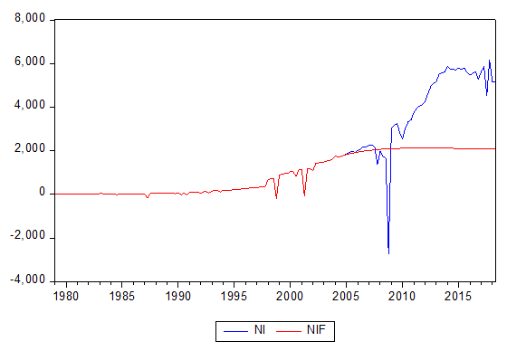
Using an ARMA (2,2) model, the quarterly data from the first quarter of 1979 up to the first quarter of 2005 are used to estimate the net income of WFC from the second quarter of 2005 to the second quarter of 2018. As the following graph shows, the unusual deviations in the actual net income from the forecasted net income could have been identified as red flags, subsequently requiring more scrutiny and investigation as well as fraud prevention.
Modeling Quarterly Net Income of West Management (WM)
Quarterly net income of West Management (WM) for periods from the first quarter of 1987 to the second quarter of 2018 is collected from the Research Insights (Compustat) data base. Figure 5 shows the plot of the quarterly net income of WM for each quarter from the first quarter of 1987 to the second quarter of 2018.
(Net Income (NI) presented in millions of dollars) Figure 5: Plot of Quarterly Net Income of WFC (1987 - 2018).
Different time series models are examined and different model selection criteria are compared. Our comparisons indicate that the first order autoregressive model and second order moving average, ARMA (1,2) best fits our observed data. Results of running ARMA (1,2) model are shown in the following table:
𝑧𝑡= 𝛽0 + 𝛽1𝑧𝑡−1 + ε𝑡+ 𝛽2ε𝑡−1 + 𝛽3ε𝑡−2 … (3) Where: 𝑧𝑡 : net income of WM in quarter t 𝑧𝑡−1 : net income of WM in quarter t - 1 ε𝑡: Residual from running the model at time t ε𝑡−1: Residual from running the model at time t - 1 ε𝑡−2: Residual from running the model at time t - 2 Table 5 summarizes the regression outputs of the Model 3, which includes data from the first quarter of 1987 to first quarter of 2018. Table 6 presents Variable Coefficient Std. Error t-Statistic Prob. C 163.1498 197.4789 0.826163 0.4104 AR(1) 0.969606 0.032959 29.41884 0 MA(1) -1.194041 0.050117 -23.82505 0 MA(2) 0.415164 0.055624 7.46374 0 SIGMASQ 51233.49 2830.861 18.0982 0 R-squared 0.292848 Mean dependent var 120.301 Adjusted R-squared 0.269078 S.D. dependent var 270.2581 S.E. of regression 231.0544 Akaike info criterion 13.77806 Sum squared resid 6352953 Schwarz criterion 13.89178 Log likelihood -849.2397 Hannan-Quinn criter. 13.82426 F-statistic 12.32015 Durbin-Watson stat 1.86809 Prob(F-statistic) 0
| AC | PAC | O-Stat | Prob |
Table 5: Summary of Regression Output of Model 3.
Autocorrelation (AC), Partial Auto Correlation (PAC), and Q-Stat as well as their significance. As shown in Table 5, the p-values (Prob.) of the coefficients of the first lag of net income, the p-value of the coefficients of the residuals from running the original models, as well as the p-value of the variable that controls for serial correlation is close to zero, indicating that these coefficients are significantly different from zero. Furthermore, the power of the test, represented by an adjusted R-Squared of 0.27, is reasonable. In addition, all model selection criteria such as Akaike Information Criterion, Schwarz Criterion, and Hannan-Quin Criterion are smaller than those of its competing models.
| AC | PAC | Q-Stat | Prob | |
| 1 | 0.213 | 0.213 | 5.7809 | 0.016 |
| 2 | 0.137 | 0.096 | 8.1817 | 0.017 |
| 3 | 0.408 | 0.381 | 29.627 | 0 |
| 4 | 0.406 | 0.32 | 51.127 | 0 |
| 5 | 0.225 | 0.126 | 57.784 | 0 |
| 6 | 0.14 | -0.074 | 60.361 | 0 |
| 7 | 0.354 | 0.115 | 77.099 | 0 |
| 8 | 0.304 | 0.078 | 89.565 | 0 |
| 9 | 0.188 | 0.069 | 94.362 | 0 |
| 10 | 0.184 | -0.01 | 99.02 | 0 |
| 11 | 0.178 | -0.112 | 103.39 | 0 |
| 12 | 0.218 | -0.019 | 110.05 | 0 |
| 13 | 0.167 | 0.022 | 113.97 | 0 |
| 14 | 0.169 | 0.067 | 118.02 | 0 |
| 15 | 0.145 | -0.012 | 121.03 | 0 |
| 16 | 0.083 | -0.122 | 122.02 | 0 |
| 17 | 0.122 | -0.065 | 124.19 | 0 |
| 18 | 0.126 | 0.024 | 126.53 | 0 |
| 19 | 0.112 | 0.083 | 128.4 | 0 |
| 20 | 0.125 | 0.101 | 130.75 | 0 |
Table 6: AC, PAC, Q-Stat, and Significance for West Management.
Using an ARMA (1,2) model, quarterly data from the first quarter of 1987 up to the first quarter of 2005 are used to estimate the net income of WM from the second quarter of 2005 to the second quarter of 2018. As the following graph shows, the unusual deviations of actual net income compare to the forecasted net income could have been identified as red flags, subsequently requiring more scrutiny and investigation as well as fraud prevention.
Concluding Remarks
As we mentioned earlier, accounting literature in time series analyses is not sufficient and this powerful tool for data analyses and forecasting is not adequately utilized in accounting and auditing. Based on our study, we believe that the accounting and auditing professions and academia are behind industries such as medicine, finance, engineering, and medical science in applying time series models. Our goal is to open the door for more studies in this area to fill accounting literature with more research to find ways through which time series models can be applied by both accounting and auditing professionals and academia. In this paper, we provide a brief definition of time series and its applications in industries such as medical science, finance, engineering, and medicine and its relevance in accounting. Time series analyses were originally used for the limited purpose of drawing a line but have developed to more advanced and complex models.
We address the use of time series models in forensic accounting by showing how time series models and analyses can be used in forensic accounting. We present three time series models as examples of applications of time series in accounting in general and forensic accounting in particular. Time series models are developed for American International Group, Wells Fargo and Company, and West Management, respectively. These three examples demonstrate how, by using appropriate time series models, fraud exposure could have been caught and prevented in a timely manner. In our three examples, we show how strongly we can explain the changes of dependent (explanatory) variables by only using the lags of the same dependent (explanatory) variables.
Our study is exploratory research that motivates future studies providing a variety of different areas in which time series analyses can be applied in accounting and auditing. We believe that accounting and auditing professionals and academics will benefit if they use time series models compare to just simply ignoring them. In addition, we believe that time series models can be embedded into a continuous audit procedure in which the model can be updated on a real time basis and used to detect major and unexpected deviations and red flags. Time series analyses enable to explain changes in the dependent variable by only using the lags of the same dependent variable, which have implications for forensic accountants investigating patters and irregularities in financial data. The accounting profession and other standards setting bodies can require companies to properly use time series models in their accounting and information systems.
Finally, as discussed earlier, we believe that this paper is the first that has identified the lack of adequate utilization of time series analyses in forensic accounting and auditing. Our paper introduces new ways in which time series analyses can be used in forensic accounting and auditing, minimizing time and cost. However, with many advantages that are discussed in this paper, come many challenges that researches should be aware of. Firstly, time series analysis is a branch of econometrics that requires special knowledge which is different from other disciplines of econometrics. Moreover, time series analysis is not available in every common or ordinary econometrics analysis software. Time series analysis can be only done in statistical analysis software such as SAS, STATA, and EViews. Secondly, time series analysis uses a vast amount of data usually for prediction and forecasting. Managing vast amounts of data can sometimes become too difficult to handle manually and requires the use of digital forensics techniques. Finally, each time series data is different from other ones and this limits the external validity or generalization of the results. In other words, a model that is developed for one company may not be appropriate for other companies.
References
-
Rezaee Z, Dorestani A, Aliabadi S (2018) Application of time series analyses in Big data: Practical, research, and education Implications. Journal of Emerging Technologies in Accounting 15(1): 183-197.
-
Ashuri B, Lu J (2010) Time Series Analysis of ENR Construction Cost Index. Journal of Constructing Engineering and Management 136(11): 1227-1237.
-
Moskowitz TJ, Ooi YH, Pedersen LH (2012) Time- Series Momentum. Journal of Financial Economics 104(2): 228-250.
-
Zakamulin V (2016) The Real-Life Performance of Market Timing with Moving Average and Time-Series Momentum Rules. The Journal of Asset Management 15(4): 261-278.
-
Baltas N, Kosowski R (2015) Demystifying Time- Series Momentum Strategies: Volatility Estimators, Trading Rules and Pairwise Correlations.
-
Rezaee Z (2019) Forensic accounting and financial statement fraud. Business Expert Press, forthcoming 2019.
-
Enders W (2015) Applied Econometrics Time Series. Wiley and Sons, Inc. New Jersey, USA. Pg no: 1-10.
-
Rice SC, Weber DP, Wu B (2015) Does SOX 404 have teeth? Consequences of the failure to Report existing internal control weaknesses. The Accounting Review 90(3): 1169-1200.
-
Association of Certified Fraud Examiners (ACFE) (2016) Report to the Nations on Occupational Fraud and Abuse.
-
Welch I (2008) The Link between Fama-French Time- Series Tests and Fama-Macbeth Cross-Sectional Tests.
-
Fama EF, French KR (1987) Commodity Futures Prices: Some Evidence on Forecast Power, Premiums, and the Theory of Storage. Journal of Business 60(1): 55-73.
-
Dudler M, Gmur B, Malamud S (2014) Risk adjusted time series momentum. Swiss Finance Institute Research Paper 14: 1-65.
-
Krahel JP, Titera WR (2015) Consequences of Big Data and Formalization on Accounting and Auditing Standards. Accounting Horizons 29(2): 409-422.
-
Amir E, Einhorn E, Kama I (2014) The role of accounting disaggregation in detecting and mitigating earnings management. Review of Accounting Studies 19(1): 43-68.
-
Yoon K, Hoogduin L, Zhang L (2015) Big Data as Complementary Audit Evidence. Accounting Horizons 29(2): 431-438.
-
Trompeter G, Wright A (2010) The world has changed-Have analytical procedure practices?. Contemporary Accounting Research 27(2): 669-700.
-
Gow ID, Ormazabal G, Taylor DJ (2010) Correcting for cross-sectional and time-series dependence in accounting research. The Accounting Review 85(2): 483-512.
-
Schipper K, Thompson R (1983) The impact of merger-related regulations on the shareholders of acquiring firms. Journal of Accounting Research 21(1): 184-221.
-
Collins DW, Dent WT (1984) A comparison of alternative testing methodologies used in capital market research. Journal of Accounting Research 22(1): 48-84.
-
Sefcik SE, Thompson R (1986) An approach to statistical inference in cross-sectional models with security abnormal returns as dependent variable. Journal of Accounting Research 24(2): 316-334.
-
Yule GU (1921) On the time-correlation problem, with special reference to the variate-difference correlation method. Journal of the Royal Statistical Society 84(4): 497-537.
-
Yule G (1926) Why do we sometimes get nonsense correlations between time series? A study in sampling and the nature of time series. Journal of the Royal Statistical Society 89(1): 1-63.
-
Yule GU (1927) On a method of investigating periodicities in disturbed series with special reference to Wolfer’s sunspot numbers. Philosophical Transactions of the Royal Society of London 226: 267- 298.
-
Alles MG, Kogan A, Vasarhelyi MA, Wu J (2006) Continuous Data Level Auditing: Business Process Based Analytic Procedures in an Unconstrained Data Environment. Working Paper, Rutgers Business School pp: 1-78.
-
Vasarhelyi MA, Alles MG, Kogan A (2004) Principles of Analytic Monitoring for Continuous Assurance. Journal of Emerging Technology in Accounting 1: 1- 21.
-
Alles MG, Kogan A, Vasarhelyi MA (2002) Feasibility and Economics of Continuous Assurance. Auditing: A Journal of Practice & Theory 21(1): 125-138.
- Forensic Implications of Adverse Drug Reactions in Schizophrenia A Case Series
- Narcotics and Digital Forensics: Bridging Crimes in the Digital Age
- Ethics in Forensic Psychiatry: Principles, Dilemmas, and Human Rights
- Impact of Acute Stress on Attentional Orienting to Social Cues
- Head Injury and Intracranial Hemorrhage in Western Region of Libya
- A Forensic Study on Handedness: Examination of Handwriting Features in Right and Left Handed Writers