Sequential Extraction and Geochemistry of Heavy Metals in Ayetoro Coastal Sediments, Southwestern Nigeria
Previous geochemical investigation of Ayetoro area discovered that its coastal sediments are enriched with sulphide mineralization. However, in order to determine the geochemical phases of the heavy metals in the coastal sediments, random sampling method was utilized across 10 locations, at a depth of 40cm using Van grab sampler at a sampling density of 200m interval. Atomic Absorption Spectrophotometer (AAS) Buck Scientific Model 205A was used to analyze nine (9) heavy metal concentrations namely Ni, Zn, Co, Mn, Fe, Pb, Cr, Cd and Cu in the coastal sediments, followed by sequential extraction of the metals, using five fractional phases. The results revealed that the geochemical concentration of the heavy metals as follows: Ni (5.89ppm - 16.82ppm), Zn (2.59ppm - 115.65ppm.), Co (1.22ppm - 22.77ppm), Mn (30.95ppm - 186.49ppm), Fe (6.632ppm - 1925.96ppm), Pb (5.17ppm - 55.96ppm), Cr (0.26ppm - 28.06ppm), Cd (0.13ppm -22.23ppm), and Cu (2.26ppm - 41.94ppm) and showed the concentration order as Residual>Reducible>Organic>Exchangeable>Carbonate. Most of the heavy metals in carbonate and exchangeable phase have low concentration except for Cd. This implied that Cd is of low mobility and bioavailability which is very dangerous as its intake by man leads to kidney diseases and causes bones to become weaker. Also, Mobility factor of Cd stood out because of its high concentration in the exchangeable phase compared to other four non-residual phases. The mobility and bioavailability of the heavy metals are in this order: Cd>Co>Ni>Pb>Cr>Mn>Cu>Zn>Fe respectively. The analysis of variance (ANOVA) revealed that the heavy metals are significantly different in all the phases based on their accumulation index in the sediments while majority of the heavy metals lacked the ability to remobilize but can be released into the environment under reducing and oxidizing conditions.
Introduction
Sediments are considered to be mixture of several components of mineral species and represent important sinks for various pollutants in aquatic systems including heavy metals. It also plays a prominent role in the assessment of heavy metal contamination [1, 2]. Total amount of heavy metal concentration in sediment is useful to detect net change.
Never the less, it does not give any sign about the chemical form of each metal in sediment [3]. Ayeku [4] studied the pollution status in the bottom sediment in Awoye, Abereke and Ayetoro Area of Ondo state. He concluded that these metals derived from the upstream rivers from the top soil are products of mechanically weathered rock materials and anthropogenic activities while Ololade [5] agreed that metal speciation should be done to determine the bioavailability of metal in sediment after his own seasonal metal distribution research in Ondo coastal sediment. Heavy metal concentration in the ocean ecosystem is determined by three conditions namely; water, sediments and living organism. Usually, heavy metal exists in lowest concentration in water and reaches considerable concentration in sediments followed by bioaccumulation in living organism. According to Li [6], heavy metals are released from sediments into water bodies and consequently, to living organisms depending on the speciation of metals and other factors such as sediment pH and organic matter [7]. Coastal and marine ecosystems worldwide are continuously bedeviled with pollution, such as eutrophication, acidification, toxic substances, heavy metals, and the likes. Decline in ecosystem productivity, loss of aesthetic beauty of the ocean, impacts on sensitive habitats, impairment on quality of seawater, hazards to human health are some of the consequences of heavy metals accumulation in sediments which makes continuous long term monitoring of heavy metal concentration of coastal sediment extremely important. Therefore, this research attempts to determine the geochemical phases of the heavy metals in the coastal sediments of Ayetoro area using five metal fractional methods, in order to assess the levels of their bioavailability, bioaccumulation and the danger it portends to man and ecology.
Description and Geology of the Study Area
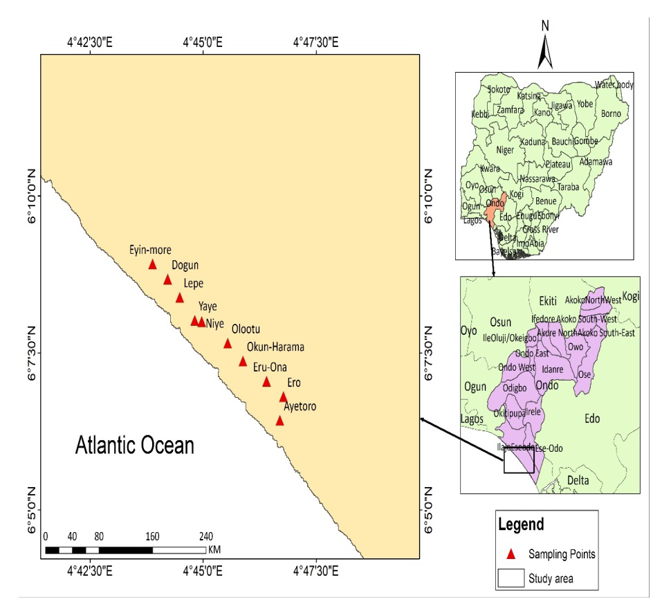
The study area (Ayetoro) is one of the prominent, water- route nodal communities in the coastal region of Ondo State, Nigeria. Ayetoro was established in 1947 and is inhabited by the Ilaje people, a linguistic subgroup of the Yorubas. The town lies east along the coast from Nigeria’s largest city, Lagos. Due to oil exploration activities, the community has lost a considerable portion of coastline to the Atlantic Ocean. Ayetoro which is one of the main settlements in Ilaje local government area lies approximately within latitude 6° 12’ 33.786” N and longitude 4° 40’ 17.051” E respectively. It is bounded in the north-east by Erunna village, on the south- east by Alagbon Village and North-west by Idi Ogba and south-west by the Atlantic Ocean. The people are extractions of the Ilaje sub-ethnic group of the Yoruba’s in south western Nigeria. Ayetoro in its hey-days once had the highest per capital income in the whole of Africa and attracted visitors, tourists and researchers from all over the world. The occupational activities in this area include fishing, canoe making, and lumbering. Others are net making, mat making, launch building, farming and trading. Residents say the ocean incursion has impacted on their livelihoods, particularly since the community’s entire mangrove vegetation was destroyed. The Atlantic’s surges have also destroyed Ayetoro’s marine life; thereby crippling people’s fishing businesses, which is the mainstay of the local economy.
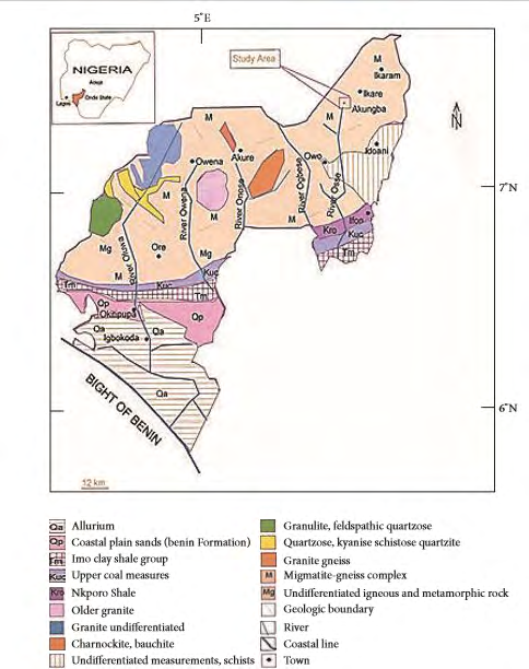
There are two distinct geological regions in Ondo State. First, is the region of sedimentary rocks in the south, and secondly, the region of Pre Cambrian-Basement Complex rocks in the north. The sedimentary rocks are mainly of the post Cretaceous sediments and the Cretaceous Abeokuta Formation. The basement complex is made up of mainly the medium-grained gneisses. These rocks are strongly foliated most of the times, occurring as outcrops. The surface of these outcrops is rigorously distorted with alternating bands of dark and light-colored minerals. These bands of light- colored minerals are essentially feldspar and quartz, while the dark colored bands contain abundant biotite, a small proportion of the state, especially to the northeast, overlies the coarse-grained granites and gneisses, which are poor in dark ferromagnesian minerals. Troughs and undulating low land surfaces cover Ilaje Local Government Area with silt, mud and superficial sedimentary deposits [8]. There are sand formation at the western part of the local government, extending from the Lekki peninsula in Lagos State to Araromi Sea-side and Zion pepe, Mahin and Ugbonla which are in the eastern part of the local government area. This could be the reason why there is sand deposition on the western side like Igbokoda and clay formation in areas like Ayetoro. Crude oil, which is a major source of income in Nigeria, is found in Ilaje Local Government. There are oil wells and fields spreading all over the local government area both onshore and offshore. Oil companies such as Shell, Chevron are believed to be presently harnessing the crude oil found in the area. Apart from petroleum, there are other natural resources and raw materials present in Ilaje land such as glass sand, salt, tar sand, quartz and clay deposits (Figures 1 & 2).
Materials and Methods
Method of Sampling and Sample collection
The samples were collected using random sampling method from Ayetoro to Eyin More. After removing the overburden, the samples were collected randomly at each station at a depth of 40cm and sample density of 200m intervals. Global Positioning Systems (GPS) G GARMIN eTrex 10 was employed to get the accurate geographical coordinates of each sampling points. A total of ten samples were collected and bagged separately inside the polythene bags and properly labelled to avoid mix up. The samples were air dried and stored in a cool and dry place to avoid contaminations. Observation of geological settings, physical structures and lithology together with human activities were noted and the samples were eventually transmitted to Temsol Consults Laboratory Ltd Shasha, Ibadan for sequential extraction analysis (Table 1).
The field data for the coastal sediment samples is presented in Table 2. Ten coastal sediments were randomly selected from different localities within the study area. Their geographical coordinates as well as their colour and nature of the sediments were taken into consideration. The colour ranges from grey, dark grey, yellowish brown, brown to brownish grey, while the composition of the sediments are clayey and silty in nature.
| Locations | Latitude | Longitude | Colour | Sediment composition | |
|---|---|---|---|---|---|
| S1 | Ayetoro | 6°6′25.76″N | 4°46′41.90″E | Dark Grey | Clay |
| S2 | Ero | 6°6′48.50″N | 4°46′46.50″E | Brownish grey | Clay |
| S3 | Eru-Ona | 6°7′3.20″N | 4°46′24.30″E | Brown | Silt |
| S4 | Okun Harama | 6°7′22.50″N | 4°45′52.80″E | Yellowish Brown | Silt |
| S5 | Olootu | 6°7′39.60″N | 4°45′32.70″E | Grey | Clay |
| S6 | Niye | 6°8′0.10″N | 4°44′58.20″E | Dark Grey | Clay |
| S7 | Yaye | 6°8′1.30″N | 4°44′48.90″E | Dark Grey | Clay |
| S8 | Lepe | 6°8′23.30″N | 4°44′29.00″E | Grey | Clay |
| S9 | Dogun | 6°8′40.78″N | 4°44′12.98″E | Grey | Clay |
| S10 | Eyin-more | 6°8′55.30″N | 4°43′53.00″E | Grey | Clay |
Table 1: Field Data and Description of Coastal Sediments.
Laboratory Analysis
Sequential Extraction Procedure
The speciation of toxic metals is important for measuring their bioavailability in the environment, and for evaluating their potential risks to living organisms [9]. In the study, the investigated metals speciation revealed differences in the concentrations that were recorded at each step of the extraction. Using a modified version of Tessier [10] method, the toxic metals were separated into five operationally defined fractions viz. exchangeable (F1), carbonate-bound (F2), Fe-Mn oxide-bound (F4), organic-bound (F4), and residual (F5) fractions (F5) [11, 12]. The sequential extraction procedures are as follows:
(i) F1: 1 g of dried and powdered sediment was extracted at room temperature with 1 M MgCl2 at pH 7.0 for 1hr with continuous agitation. Then, the mixture was centrifuged. The supernatant obtained on standing was filtered to represent F1.
(ii) F2: The residue from (i) was leached at 30 ºC with 1 M sodium acetate (NaOAc) adjusted to pH 5.0 with acetic acid (HOAc). The mixture was continuously agitated throughout the extraction using a centrifuge. The extracts were decanted to represent F2.
(iii) F3: 20 ml of 0.04 M hydroxylamine chloride (NH2OH. HCl) in 25% (v/v) acetic was added to the residue from (ii). The mixture was agitated 96°C for 6 h. Then, the extract was decanted to represent F3.
(iv) F4: 3ml of 0.02 M HNO3 and 5ml of 30% H2O2 were added to the residue from (iii). The mixture was agitated at 85°C for 5 hours then, 5 ml of 3.2 M NH4OAc was added and further centrifuging for 30 min before filtering. The supernatant represents F4.
(v) F5: The final fraction was obtained by digesting the residual from (iv) with 5ml of 25% of HC1 and 5ml HNO3. for 6hrs at 120°C. The mixture was centrifuged, and the supernatant was obtained as F5.
All reagents used were analytical grade. The supernatant from each extraction was quantitatively transferred into a 25 ml volumetric flask and made up to mark with 1 M HNO3 before quantifying the trace metals using Atomic Absorption Spectrophotometer (AAS, Buck Scientific Model 205A). All analyses were carried out in triplicates, and reagent blanks were used for quality control.
Metal Analysis
Trace metal concentrations were determined by atomic absorption spectrophotometry Model 210 VGP of the Buck Scientific AAS series with air-acetylene gas mixture as oxidant involving direct aspiration of the aqueous solution into an air-acetylene flame. The following techniques were used for the first four fractions. For the trace metals Cd, Co, Cu, Cr Ni, Pb, and Zn, For the metals present in high concentrations (Fe and Mn) the supernatant solution was diluted (20 to 50 X) with deionized water and the concentrations were obtained directly from appropriate calibration curves prepared with the components of the extraction solution diluted by the same factor. For total or residual trace metal analysis, the solid was digested with a 5:1 mixture of hydrofluoric and perchloric acids. For 1g (dry weight) sample, the sediment was first digested in a platinum crucible with a solution of concentrated HC104 (2 ml) and HF (10 ml) to near dryness; subsequently, a second addition of HC104 (1 ml) and HF (10 ml) was made and again the mixture was evaporated to near dryness. Finally, HC104 (1 ml) alone was added and the sample was evaporated until the appearance of white fumes. The residue was dissolved in 12ml NHC1 and diluted to 25 ml. The resulting solution was then analyzed by flame atomic absorption spectrophotometry for trace metals using the standard addition techniques.
$$ \frac {\mathrm {F 1} + \mathrm {F 2}}{\mathrm {F 1} + \mathrm {F 2} + \mathrm {F 3} + \mathrm {F 4} + \mathrm {F 5}} * 1 0 0 $$ Mobility Factor= Mobility Factor is used to evaluate the potential mobility of and bioavailability of heavy metal. High percentage represents high potential and vice versa
Results and Discussion
Geochemical Phases
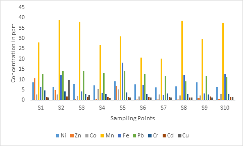
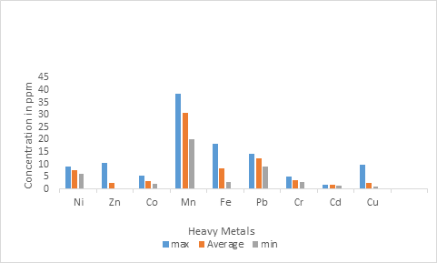
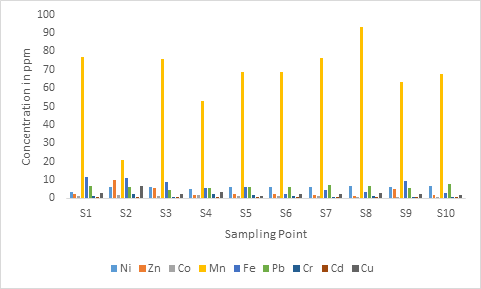
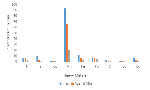
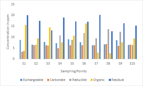
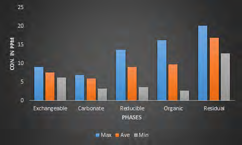
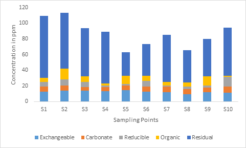
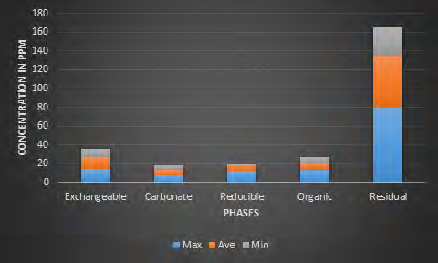
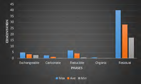
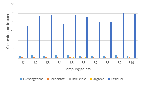
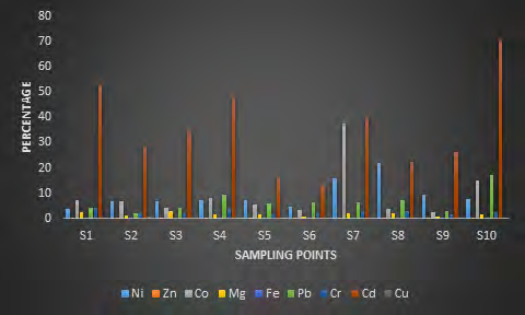
Exchangeable Phase Table 5 showed the distribution of the maximum, average and minimum concentration of nine heavy metals in the exchangeable phase. The average concentration of the heavy metals is: Mn>Pb>Fe>Ni>Cr>Co>Zn>Cu>Cd. Also, Figures 3 and 4 showed that Mn is predominantly abundant across all sampling points. The following are the range of concentration of heavy metals in this phase: Ni (6.24 – 9.04), Zn (0.07 – 10.64), Co (1.9 – 5.42), Mn (20.16 - 38.72), Fe (2.64 – 18.32), Pb (9.04 – 14.32), Cr (2.72 – 4.85), Cd (1.29 – 1.74), Cu (0.96 -9.76). Apart from sample point S1, Zn is notably low in all other points. Conc. of Fe in S2, S5 and S10 are notably different from others perhaps because of inflow of some extraneous materials from the land to this particular area.
| Toxic Metals | Ni | Zn | Co | Mn | Fe | Pb | Cr | Cd | Cu |
|---|---|---|---|---|---|---|---|---|---|
| Max conc.(ppm) | 9.04 | 10.64 | 5.42 | 38.72 | 18.32 | 14.32 | 4.85 | 1.74 | 9.76 |
| Average conc.(ppm) | 7.52 | 2.59 | 3.10 | 30.95 | 8.29 | 12.51 | 3.38 | 1.57 | 2.26 |
| Min conc.(ppm) | 6.24 | 0.07 | 1.9 | 20.16 | 2.64 | 9.04 | 2.72 | 1.29 | 0.96 |
Table 2: Maximum, Average and Minimum Concentration of heavy metals in the Exchangeable phase.
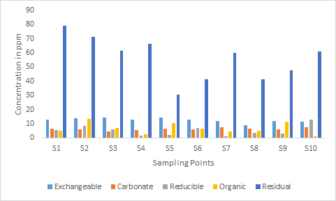
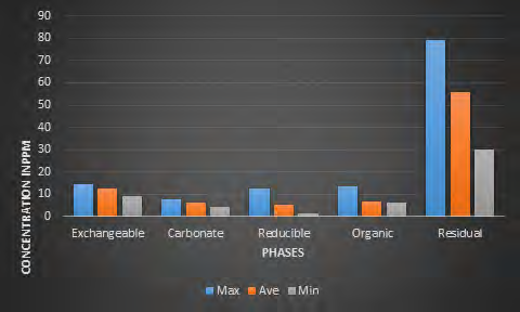
Carbonate Phase Table 3 presents the distribution of the maximum, average and minimum concentration of nine heavy metals in the carbonate phase. Average concentration of the heavy metals are in this order: Mn>Fe > Pb >Ni>Zn > Cu>Cr>Co > Cd. The average concentration of Fe is a little higher than Pb in the carbonate phase unlike the exchangeable phase. Likewise, the average concentration of Zn is higher than Cr in the carbonate phase. Except for Zn and Mn the average concentration of all the other heavy metals reduce drastically in the carbonate phase. The following are the ranges of concentration of heavy metals in this phase. Ni (3.25 -6.81), Zn (1.33 – 9.71), Co (0.37 – 1.72), Mn (20.72 – 93.36), Fe (2.08 -11.68), Pb (4.56 – 7.62), Cr (0.12 – 2.3), Cd (0.54 – 0.94), Cu (1.44 - 6.72) (Figures 5 and 6 respectively).
| Heavy Metals | Ni | Zn | Co | Mn | Fe | Pb | Cr | Cd | Cu |
|---|---|---|---|---|---|---|---|---|---|
| Max conc.(ppm) | 6.81 | 9.71 | 1.72 | 93.36 | 11.68 | 7.62 | 2.3 | 0.94 | 6.72 |
| Ave conc.(ppm) | 5.894 | 3.37 | 1.222 | 66.55 | 6.632 | 6.278 | 1.162 | 0.743 | 2.854 |
| Min conc.(ppm) | 3.25 | 1.33 | 0.37 | 20.72 | 2.08 | 4.56 | 0.12 | 0.54 | 1.44 |
Table 3: Maximum, average and minimum concentration of heavy metals in the carbonate phase.
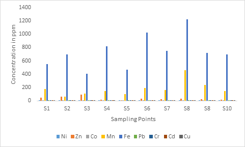
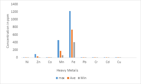
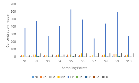
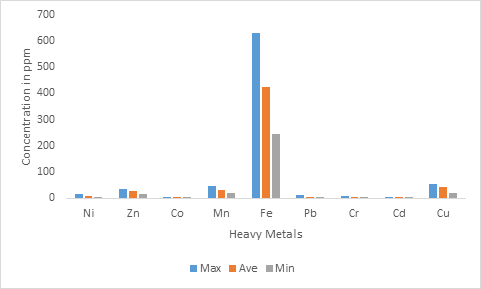
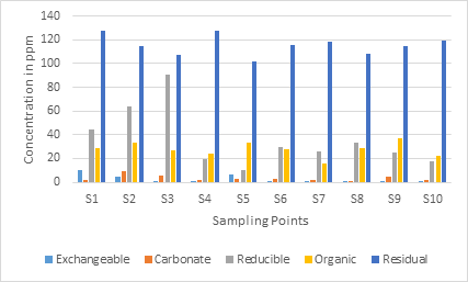
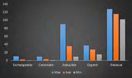
Reducible Phase Table 4 presents the distribution of the maximum, average and minimum concentration of nine heavy metals in the Reducible phase. Average concentration of the heavy metals is in this order: Fe> Mn> Zn> Ni> Cu>Pb> Co> Cr> Cd. The concentrations of Fe and Mn have tremendously increased to more than 50% for Mn and 100% for Fe respectively (Figures 7 and 8). Except for Pb and Cd, the concentration of all other metals increases notably since the previous phase. The following are the ranges of concentration of heavy metal in this phase: Ni (3.66 -13.6), Zn (10.12 – 90.64), Co (1.87 – 9.12), Mn (60.76 – 463.4), Fe (409.89 – 1222.14), Pb (1.34 – 12.8), Cr (0.83 – 6.48), Cd (0.02 – 0.22), Cu (2.23 -12.27).
| Heavy Metals | Ni | Zn | Co | Mn | Fe | Pb | Cr | Cd | Cu |
|---|---|---|---|---|---|---|---|---|---|
| Max conc.(ppm) | 13.6 | 90.64 | 9.12 | 463.4 | 1222.14 | 12.8 | 6.48 | 0.22 | 12.27 |
| Ave conc.(ppm) | 8.98 | 35.959 | 5.093 | 178.867 | 735.334 | 5.165 | 4.233 | 0.128 | 5.99 |
| Min conc.(ppm) | 3.66 | 10.12 | 1.87 | 60.76 | 409.89 | 1.34 | 0.83 | 0.02 | 2.23 |
Table 4: Maximum, Average and Minimum Concentration of heavy metals in the Reducible phase.
Organic Phase The distribution of the maximum, average and minimum concentration of nine heavy metals in organic phase is presented (Table 5). Average concentration of the heavy metals is in this order: Fe> Cu> Mn> Zn> Ni> Pb> Cr>Cd >Co. The average concentration of Cu over the sampling points in the organic phase increased drastically (Figures 9 and 10).
| Heavy Metals | Ni | Zn | Co | Mn | Fe | Pb | Cr | Cd | Cu |
|---|---|---|---|---|---|---|---|---|---|
| Max conc.(ppm) | 16.21 | 37.34 | 5.62 | 47.04 | 628.59 | 13.6 | 9.52 | 0.62 | 55.21 |
| Ave conc.(ppm) | 9.66 | 27.75 | 2.809 | 31.058 | 424.267 | 6.776 | 6.408 | 0.26 | 41.939 |
| Min conc.(ppm) | 2.69 | 15.8 | 0.74 | 19.46 | 245.18 | 1.29 | 2.71 | 0.04 | 21.26 |
Table 5: Maximum, average and minimum Concentration of heavy metals in the Organic Phase.
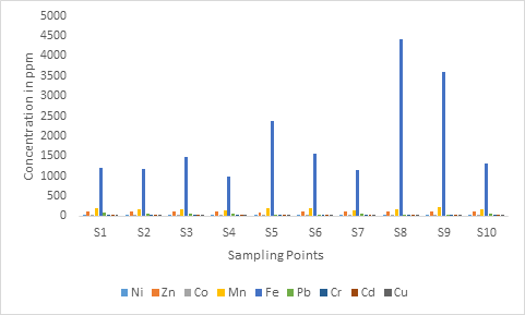
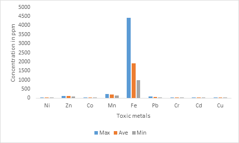
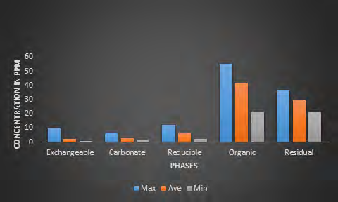
Residual Phase Table 6 presents the distribution of the maximum, average and minimum concentration of nine heavy metals in the residual phase. Average concentration of the heavy metals is in this order: Fe> Mn> Zn> Pb> Cu> Cr> Co >Cd Ni. Fe has the highest concentration in this phase (Figures 11and 12).
| Toxic Metals | Ni | Zn | Co | Mn | Fe | Pb | Cr | Cd | Cu |
|---|---|---|---|---|---|---|---|---|---|
| Max conc.(ppm) | 20.15 | 127.51 | 29.65 | 230.22 | 4412.61 | 79.2 | 40.05 | 25.1 | 36.64 |
| Ave conc.(ppm) | 16.819 | 115.647 | 22.7795 | 186.498 | 1925.966 | 55.963 | 28.055 | 22.228 | 29.434 |
| Min conc.(ppm) | 12.66 | 102.22 | 2.715 | 155.65 | 1000.95 | 30.3 | 17.14 | 17.85 | 21.16 |
Table 6: Maximum, Average and Minimum Concentration of Heavy metals in the Residual Phase.
Analysis of Heavy Metals Across all Phases
Nickel (Ni) The average concentration of Ni over the sampling points and across all phases is between 5.89ppm to 16.82ppm (Table 7). The concentration increases in this order; Resi dual>Organic>Reducible>Exchangeable>Carbonate. Ni is predominantly abundant in the residual and organic phases, except for S7 and S8 (Figures 13 and 14) which have low concentration in the organic phase. This means that it is of mineral origin and do not pose any biological risk. Ni plays an important role in the development of some plants. However, it is not an essential nutrient for human. However, the kidney removes most of the nickel absorbed by humans.
| Phases | Max | Ave | Min |
|---|---|---|---|
| Exchangeable | 9.04 | 7.52 | 6.24 |
| Carbonate | 6.81 | 5.89 | 3.25 |
| Reducible | 13.6 | 8.98 | 3.66 |
| Organic | 16.21 | 9.66 | 2.69 |
| Residual | 20.15 | 16.82 | 12.66 |
Table 7: Maximum, Average and Minimum Concentration. Of Ni Over all Phases.
Zinc (Zn) The average concentration of Zn over the sampling points and across all phases is between 2.59ppm to 115.65ppm (Table 8). The concentration increases in this order; Residual> Reducible>Organic>Carbonate>Exchange able. Zinc is mostly abundant in the residual phase and S1 and S4 have the highest concentrations while it is of high concentration in other phases. For instance, sampling points such as S3, S4, S6, S7, S8 and S10 showed that it is low in the exchangeable phase. Zinc is an important element in the environment. Its deficiency is connected to many diseases such as delayed sexual maturation, infection susceptibility and diarrhea. Zinc is important for over 300 enzymes and 1000 transcription factors, and is stored and transferred in metallothioneins. Excess zinc is however toxic to plants. Fishes cannot tolerate the amount of Zn, as do plants [13]. Excess zinc inhibits calcium uptake in fish, which can be deadly (Figures 15 and 16). In this study, it is discovered that the concentration of Zn exceeded the normal concentration expected to be in sediment hence this necessitates prompt measures to curtail its menace.
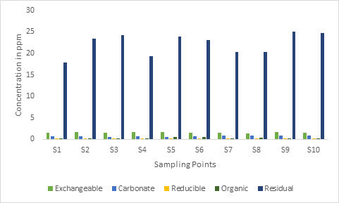
Cobalt (Co) The average concentration of Co over the sampling points and across all phases is between 1.22ppm to 22.77ppm respectively (Table 8). The concentration increases in this order; Residual> Reducible>Exchangeable>Carbonate>O rganic. Co is mostly abundant in the Residual phase and relatively low in other phases with S1 having the highest concentration (Figures 17 and 18). Co is always involved in photosynthesis and nitrogen fixation detected in most ocean basins and a limiting micronutrient for phytoplanktons and cyanobacteria. P value of 5.71E-17 in analysis of variance indicated that there is a significant difference from one phase to another.
| Phases | Max | Ave | Min |
|---|---|---|---|
| Exchangeable | 5.42 | 3.09 | 1.9 |
| Carbonate | 1.72 | 1.22 | 0.37 |
| Reducible | 9.12 | 5.09 | 1.87 |
| Organic | 5.62 | 2.80 | 0.74 |
| Residual | 29.65 | 22.77 | 2.72 |
Table 8: Maximum, Average and Minimum concentration of Co over all the Phases
Manganese (Mn) The average concentration of Mn over the sampling points and across all phases is between 30.95ppm to 186.49ppm (Table 9). The concentration increases in this order; Residual> Reducible> Carbonate Organic>Exchangeable. Except for sampling point S8, which has an extremely high concentration in the reducible phase, Mn is evenly abundant in the residual phase followed by the reducible phase. In the aquatic bodies, many enzymatic systems need Mn to function, but in high levels, Mn can become toxic. At level of 500ppm Mn is dangerous to life; therefore Mn in the study area does not pose any threat to lives in the location. 3.2E-10 P value of annova indicates that there is significant difference between the five phases (Figures 19 and 20).
| Phases | Max | Ave | Min |
|---|---|---|---|
| Exchangeable | 38.72 | 30.95 | 20.16 |
| Carbonate | 93.36 | 66.55 | 20.72 |
| Reducible | 463.4 | 178.86 | 60.76 |
| Organic | 47.04 | 31.06 | 19.46 |
| Residual | 230.22 | 186.49 | 155.65 |
Table 9: Maximum, Average and Minimum concentration of Mn over all the Phases.
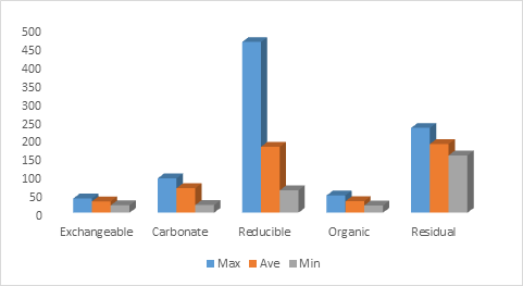
Iron (Fe) According to Table 10, the average concentration of Fe over the sampling points and across all phases is between 6.632ppm to 1925.96ppm. The concentration increases in this order; Residual> Reducible > Organic>Exchangeable>Carbonate (Figures 21 and 22). Iron is extremely low in the carbonate and exchangeable phase but very high in the residual and also present in the reducible phase. Iron accumulation poses a problem for aerobic organisms because ferric iron is poorly soluble near neutral ph. Iron plays an essential role in marine systems and can act as a limiting nutrient for planktonic activity. Its excess may lead to a decrease in growth rates in phytoplantonic organisms. 5.6E-10 P value of ANOVA indicates that there is significant difference between the five phases.
| Phases | Max | Ave | Min |
|---|---|---|---|
| Exchangeable | 18.32 | 8.29 | 2.64 |
| Carbonate | 11.68 | 6.632 | 2.08 |
| Reducible | 1222.14 | 735.33 | 409.89 |
| Organic | 628.59 | 424.27 | 245.18 |
| Residual | 4412.6 | 1925.96 | 1000.95 |
Table 10: Maximum, Average, minimum concentration of Fe over the mineralogical Phases.
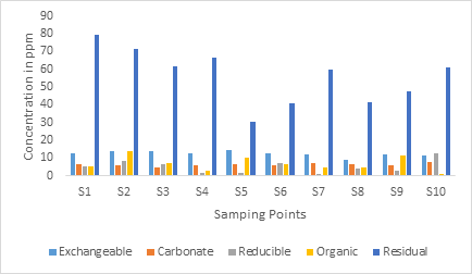
Lead (Pb) Table 11 presents the average concentration of Pb over the sampling points and across all phases to be between 5.17ppm to 55.96ppm. The concentration increases in this order; Residual> Exchangeable> Organic >Carbonate>Reducible (Figures 23 and 24). Pb is more abundant in the Residual phase and has no confirmed safe level of exposure. Even at level considered to pose little or no risk, Pb may cause adverse mental health outcomes. Pb is a highly poisonous metal both inhaled and swallowed, causing great damage to almost every organs and systems in the human body. High level of Pb causes lead poisoning while low levels cause increase susceptibility to terminal diseases. High concentration of lead has the capacity to inhibit photosynthesis. Bioaccumulation of Pb poses a serious hazard to fishes and other sea mammals. From the results obtained in this study, the concentration is within the residual phase which means that Pb is not bioavailable and will therefore tend not to remobilize. 9.5E-21 P value of ANOVA indicated that there is significant difference between five phases.
| Phases | Max | Ave | Min |
|---|---|---|---|
| Exchangeable | 14.32 | 12.51 | 9.04 |
| Carbonate | 7.62 | 6.28 | 4.56 |
| Reducible | 12.8 | 5.17 | 1.34 |
| Organic | 13.6 | 6.78 | 6.41 |
| Residual | 79.2 | 55.96 | 30.3 |
Table 11: Maximum, Average and Minimum concentration of Pb over all the Phases.
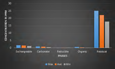
Chromium (Cr) The result of the average concentration of Cr over the sampling points and across all phases is between 0.26ppm to 28.06ppm (Table 12). The concentration increases in this order; Residual >Reducible>Exchangeable>Carbonate>Orga nic. Cr is more abundant in the residual phase and extremely low in the organic phase (Figures 25 and 26). Chromium is highly toxic to fish because it is easily absorbed across gills, readily enters blood circulation, and crosses cell membrane and bio concentrate up the food chain. Acute and chronic exposure to chromium affects fish behavior, physiology, reproduction and survival. Toxicity ranges between 50 and 150 ppm [14]. 1.07E-20 P value of ANOVA indicates that there is significant difference between five phases.

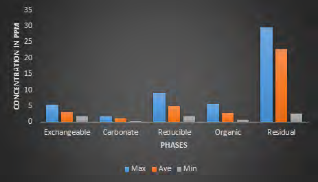
Cadmium (Cd) Table 12 revealed that the average concentration of Cd over the sampling points and across all phases is between 0.13ppm to 22.23ppm. The concentration increases in this order; Residual> Exchangeable> Carbonate>Organic > Reducible. Cd is abundant in the residual and present in an extremely low concentration in other phases (Figures 27and 28) respectively. Cd is considered an environmental pollutant that causes health hazards to living organisms. Anthropogenic sources include fossils fuel combustion and fertilizers. Cd exposure is associated with a large number of illnesses including kidney disease, early atherosclerosis, hypertension and cardiovascular diseases. 5.11E-40 P value of annova indicates that there is significant difference between five phases. Cd in this location must be monitored because it has good percentage of its concentration in the exchangeable phase [15].
| Phases | Max | Ave | Min | |
|---|---|---|---|---|
| Exchangeable | 1.74 | 1.57 | 1.29 | |
| Carbonate | 0.94 | 0.74 | 0.54 | |
| Reducible | 0.22 | 0.13 | 0.02 | |
| Organic | 0.62 | 0.26 | 0.04 | |
| Residual | 25.1 | 22.23 | 17.85 |
Table 12: Maximum, Average and Minimum Concentration of Cd over all the Phases.
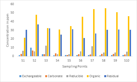
Cupper (Cu) The average concentration of Cu over the sampling points and across all phases is between 2.26ppm to 41.94ppm (Table 13). The concentration increases in this order; Organic> Residual > Carbonate>Reducible. Cu is more abundant in the organic phase (Figures 29 and 30). Due to its role in facilitating iron uptake, Cu deficiency can produce anemia-like systems, neutropenia, bone abnormalities and impaired growth. 2.4E-27 P value of annova indicates that there is significant difference between the five phases.
| Phases | Max | Ave | Min |
|---|---|---|---|
| Exchangeable | 9.76 | 2.26 | 0.96 |
| Carbonate | 6.72 | 2.85 | 1.44 |
| Reducible | 12.27 | 5.99 | 2.33 |
| Organic | 55.21 | 41.94 | 21.26 |
| Residual | 36.64 | 29.43 | 21.16 |
Table 13: Maximum, Average and Minimum concentration of Cu over all the Phases.
Mobility Factor across the Metal fractional phases
The mobility factors of the various heavy metals analyzed is presented in Tables 14-22. It can be deduced that Cd has the highest potential to remobilize across all sampling points because of its high mobility factor (Figure 31).
| Sample Points | F1 | F2 | F3 | F4 | F5 | Mobility Factor(%) |
|---|---|---|---|---|---|---|
| S1 | 8.72 | 3.25 | 3.66 | 15.6 | 20.01 | 3.65 |
| S2 | 6.56 | 6.32 | 6.57 | 9.39 | 17.42 | 7.04 |
| S3 | 7.84 | 6.24 | 6.22 | 14.41 | 13.05 | 6.76 |
| S4 | 7.28 | 4.88 | 10.8 | 7.67 | 19 | 7.21 |
| S5 | 9.04 | 6.24 | 8.81 | 10.64 | 17.2 | 7.38 |
| S6 | 7.68 | 6.32 | 11.86 | 16.21 | 17.05 | 4.63 |
| S7 | 6.24 | 6.32 | 9.43 | 2.85 | 20.15 | 15.82 |
| S8 | 6.72 | 6.81 | 13.6 | 2.69 | 12.66 | 22.11 |
| S9 | 8.64 | 6 | 12.44 | 7.66 | 16.35 | 9.61 |
| S10 | 6.48 | 6.56 | 6.41 | 9.48 | 15.3 | 7.93 |
Table 14: Mobility Factor of Ni.
| Sampling Points | F1 | F2 | F3 | F4 | F5 | Mobility Factor (%) |
|---|---|---|---|---|---|---|
| S1 | 10.64 | 2.07 | 44.26 | 28.51 | 127.51 | 0.34 |
| S2 | 4.96 | 9.71 | 64.02 | 33.42 | 115.05 | 0.37 |
| S3 | 0.59 | 5.71 | 90.64 | 27.22 | 107.57 | 0.21 |
| S4 | 0.48 | 1.66 | 19.34 | 23.72 | 127.25 | 0.07 |
| S5 | 6.96 | 2.46 | 10.12 | 33.51 | 102.22 | 0.27 |
| S6 | 0.16 | 2.46 | 29.74 | 27.62 | 115.71 | 0.08 |
| S7 | 0.41 | 1.74 | 25.86 | 15.8 | 118.55 | 0.11 |
| S8 | 0.07 | 1.33 | 33.34 | 28.58 | 108.58 | 0.04 |
| S9 | 1.07 | 4.85 | 24.64 | 37.34 | 115.09 | 0.14 |
| S10 | 0.53 | 1.71 | 17.63 | 21.78 | 118.94 | 0.09 |
Table 15: Mobility Factor of Zn.
| Sampling Points | F1 | F2 | F3 | F4 | F5 | Mobility Factor (%) |
|---|---|---|---|---|---|---|
| S1 | 2.88 | 1.46 | 3.34 | 1.82 | 29.35 | 7.10 |
| S2 | 2.84 | 1.68 | 1.87 | 2.15 | 27.25 | 6.95 |
| S3 | 2.09 | 1.26 | 3.38 | 2.42 | 29.65 | 4.26 |
| S4 | 5.42 | 1.72 | 6.92 | 2.96 | 25.25 | 8.04 |
| S5 | 5.31 | 1.34 | 3.24 | 4.18 | 26.75 | 5.46 |
| S6 | 1.9 | 1.26 | 8.76 | 4.04 | 21.08 | 3.25 |
| S7 | 2.75 | 1.29 | 4.12 | 0.98 | 2.715 | 37.33 |
| S8 | 2.3 | 0.95 | 9.12 | 3.18 | 23.18 | 3.77 |
| S9 | 2.34 | 0.89 | 6.28 | 5.62 | 21.41 | 2.48 |
| S10 | 3.13 | 0.37 | 3.9 | 0.74 | 21.16 | 15.17 |
| S1 | 28.08 | 76.88 | 180.21 | 19.52 | 205.18 | 2.44 |
| S2 | 38.72 | 20.72 | 60.76 | 30.01 | 175.46 | 1.10 |
| S3 | 38.08 | 76.08 | 107.55 | 19.46 | 175.23 | 3.14 |
| S4 | 26.88 | 53.21 | 143.81 | 31.74 | 155.82 | 1.54 |
| S5 | 30.88 | 68.8 | 100.26 | 29.73 | 210.02 | 1.54 |
| S6 | 20.72 | 68.82 | 190.62 | 47.04 | 205.11 | 0.90 |
| S7 | 20.16 | 76.48 | 158.86 | 25.67 | 155.65 | 2.27 |
| S8 | 38.64 | 93.36 | 463.4 | 31.4 | 171.45 | 2.20 |
| S9 | 29.68 | 63.23 | 236.6 | 42.81 | 230.22 | 0.91 |
| S10 | 37.68 | 67.92 | 146.6 | 33.2 | 180.84 | 1.68 |
Table 16: Mobility Factor of Co.
| Sampling Points | F1 | F2 | F3 | F4 | F5 | Mobility Factor (%) |
|---|---|---|---|---|---|---|
| S1 | 6.38 | 11.68 | 552.04 | 381.62 | 1196.8 | 0.003 |
| S2 | 12.16 | 11.22 | 694.3 | 481.08 | 1185.45 | 0.004 |
| S3 | 4.16 | 8.88 | 409.89 | 278.84 | 1484.5 | 0.003 |
| S4 | 3.44 | 5.76 | 816.28 | 412.18 | 1000.95 | 0.002 |
| S5 | 18.32 | 6.08 | 470.9 | 628.59 | 2372.65 | 0.001 |
| S6 | 7.44 | 2.08 | 1023.8 | 495.08 | 1555.3 | 0.001 |
| S7 | 2.64 | 4.46 | 746.5 | 245.18 | 1145.15 | 0.002 |
| S8 | 12.24 | 3.52 | 1222.14 | 441.42 | 4412.61 | 0.0008 |
| S9 | 3.24 | 9.68 | 718.87 | 600 | 3591.2 | 0.0005 |
| S10 | 12.88 | 2.96 | 698.62 | 278.68 | 1315.05 | 0.004 |
Table 17: Mobility Factor of Fe.
| Sampling Points | F1 | F2 | F3 | F4 | F5 | Mobility Factor(%) |
|---|---|---|---|---|---|---|
| S1 | 12.88 | 6.56 | 5.49 | 5.22 | 79.2 | 4.43 |
| S2 | 14.01 | 6.12 | 8.44 | 13.6 | 71.15 | 2.02 |
| S3 | 14.16 | 4.56 | 6.25 | 7.02 | 61.6 | 4.09 |
| S4 | 12.96 | 5.76 | 1.56 | 2.68 | 66.4 | 9.44 |
| S5 | 14.32 | 6.32 | 1.88 | 10.42 | 30.3 | 6.10 |
| S6 | 12.8 | 6.08 | 7.21 | 6.46 | 41.1 | 6.47 |
| S7 | 11.76 | 7.36 | 1.34 | 4.64 | 59.85 | 6.41 |
| S8 | 9.04 | 6.56 | 3.81 | 4.82 | 41.18 | 7.15 |
| S9 | 11.84 | 5.84 | 2.87 | 11.61 | 47.85 | 3.06 |
| S10 | 11.36 | 7.62 | 12.8 | 1.29 | 61 | 17.18 |
| S1 | 4.85 | 1.34 | 4.76 | 5.84 | 22.05 | 4.43 |
| S2 | 4.12 | 2.3 | 2.14 | 9.36 | 28.54 | 2.32 |
| S3 | 3.08 | 0.96 | 6.24 | 5.12 | 38.35 | 1.95 |
| S4 | 2.96 | 2.24 | 5.26 | 4.5 | 26.41 | 4.02 |
| S5 | 3.66 | 1.54 | 6.48 | 8.63 | 32.56 | 1.77 |
| S6 | 3.11 | 1.17 | 4.44 | 6.58 | 29.95 | 2.07 |
| S7 | 3.22 | 0.51 | 5.68 | 2.71 | 40.05 | 3.16 |
| S8 | 3.04 | 1.12 | 3.94 | 7.14 | 17.14 | 3.18 |
| S9 | 2.72 | 0.32 | 2.56 | 9.52 | 18.05 | 1.71 |
| S10 | 3.06 | 0.12 | 0.83 | 4.68 | 27.45 | 2.40 |
Table 18: Mobility Factor of Pb.
| Sampling Points | F1 | F2 | F3 | F4 | F5 | Mobility Factor (%) |
|---|---|---|---|---|---|---|
| S1 | 1.55 | 0.75 | 0.12 | 0.11 | 17.85 | 52.46 |
| S2 | 1.74 | 0.66 | 0.15 | 0.25 | 23.35 | 28.61 |
| S3 | 1.58 | 0.54 | 0.16 | 0.16 | 24.19 | 34.46 |
| S4 | 1.62 | 0.65 | 0.13 | 0.12 | 19.34 | 48.08 |
| S5 | 1.66 | 0.61 | 0.19 | 0.48 | 23.94 | 16.27 |
| S6 | 1.52 | 0.73 | 0.22 | 0.62 | 23.13 | 13.38 |
| S7 | 1.52 | 0.94 | 0.11 | 0.18 | 20.25 | 39.58 |
| S8 | 1.29 | 0.85 | 0.14 | 0.36 | 20.36 | 22.26 |
| S9 | 1.67 | 0.82 | 0.02 | 0.28 | 25.1 | 26.10 |
| S10 | 1.55 | 0.88 | 0.04 | 0.04 | 24.77 | 70.21 |
Table 19: Mobility factor of Cd.
| Sampling Points | F1 | F2 | F3 | F4 | F5 | Mobility Factor (%) |
|---|---|---|---|---|---|---|
| S1 | 1.36 | 2.64 | 6.29 | 21.26 | 30.43 | 0.60 |
| S2 | 9.76 | 6.72 | 5.81 | 47.83 | 36.64 | 0.92 |
| S3 | 2.48 | 2.41 | 12.27 | 32.49 | 32.04 | 0.46 |
| S4 | 0.96 | 3.44 | 2.23 | 30.88 | 24.82 | 0.56 |
| S5 | 1.28 | 1.44 | 2.26 | 34.64 | 31.18 | 0.25 |
| S6 | 1.36 | 2.48 | 5.81 | 45.62 | 21.16 | 0.39 |
| S7 | 1.36 | 2.08 | 11.4 | 54.4 | 26.34 | 0.24 |
| S8 | 1.22 | 2.85 | 4.2 | 55.21 | 30.36 | 0.24 |
| S9 | 1.36 | 2.56 | 4.21 | 50.86 | 30.95 | 0.25 |
| S10 | 1.52 | 1.92 | 5.42 | 46.2 | 30.42 | 0.24 |
Table 20: Mobility factor of Cu.
Statistical Analysis
Analysis of Variance (ANNOVA)
The analysis of variance using single factor for the geochemical phases between and within the geochemical groups are presented in Tables 23-31 using SPSS IBM 15. The results showed that there are no significant variations between the metals except cadmium but there are significant variations between and within the groups of geochemical speciation.
| SUMMARY | ||||||
|---|---|---|---|---|---|---|
| Groups | Count | Sum | Average | Variance | ||
| Exchangeble Phase | 10 | 75.2 | 7.52 | 1.052444 | ||
| Carbonate Phase | 10 | 58.94 | 5.894 | 1.121849 | ||
| Reducible Phase | 10 | 89.8 | 8.98 | 10.38747 | ||
| Organic Phase | 10 | 96.6 | 9.66 | 22.74793 | ||
| Residual Phase | 10 | 168.19 | 16.819 | 6.736054 | ||
| ANOVA | ||||||
| Source of Variation | SS | df | MS | F | P-value | F crit |
| Between Groups | 704.1037 | 4 | 176.0259 | 20.93267 | 8.39E-10 | 2.578739 |
| Within Groups | 378.4117 | 45 | 8.40915 | |||
| Total | 1082.515 | 49 | ||||
| Groups | Count | Sum | Average | Variance | ||
| Exchangeable Phase | 10 | 25.87 | 2.587 | 13.50333 | ||
| Carbonate Phase | 10 | 33.7 | 3.37 | 7.078444 | ||
| Reducible Phase | 10 | 359.59 | 35.959 | 600.1978 | ||
| Organic Phase | 10 | 277.5 | 27.75 | 39.28258 | ||
| Residual Phase | 10 | 1156.47 | 115.647 | 65.64078 | ||
| ANOVA | ||||||
| Source of Variation | SS | df | MS | F | P-value | F crit |
| Between Groups | 85872.09 | 4 | 21468.02 | 147.9119 | 2.82E-25 | 2.578739 |
| Within Groups | 6531.326 | 45 | 145.1406 | |||
| Total | 92403.41 | 49 |
Table 21: Ni.
| SUMMARY | ||||||
|---|---|---|---|---|---|---|
| Groups | Count | Sum | Average | Variance | ||
| Exchangeable Phase | 10 | 30.96 | 3.096 | 1.575938 | ||
| Carbonate Phase | 10 | 12.22 | 1.222 | 0.160662 | ||
| Reducible Phase | 10 | 50.93 | 5.093 | 6.289912 | ||
| Organic Phase | 10 | 28.09 | 2.809 | 2.294099 | ||
| Residual Phase | 10 | 227.795 | 22.7795 | 60.26222 | ||
| ANOVA | ||||||
| Source of Variation | SS | Df | MS | F | P-value | F crit |
| Between Groups | 3188.203 | 4 | 797.0506 | 56.46207 | 5.71E-17 | 2.578739 |
| Within Groups | 635.2455 | 45 | 14.11657 | |||
| Total | 3823.448 | 49 |
Table 22: Co.
| SUMMARY | ||||||
|---|---|---|---|---|---|---|
| Groups | Count | Sum | Average | Variance | ||
| Exchangeable Phase | 10 | 309.52 | 30.952 | 51.45948 | ||
| Carbonate Phase | 10 | 665.5 | 66.55 | 368.4856 | ||
| Reducible Phase | 10 | 1788.67 | 178.867 | 12479.66 | ||
| Organic Phase | 10 | 310.58 | 31.058 | 77.58173 | ||
| Residual Phase | 10 | 1864.98 | 186.498 | 617.8134 | ||
| ANOVA | ||||||
| Source of Variation | SS | df | MS | F | P-value | F crit |
| Between Groups | 243340.5 | 4 | 60835.14 | 22.37409 | 3.20E-10 | 2.578739 |
| Within Groups | 122355 | 45 | 2719 | |||
| Total | 365695.5 | 49 | ||||
| Groups | Count | Sum | Average | Variance | ||
| Exchangeable Phase | 10 | 82.9 | 8.29 | 28.29149 | ||
| Carbonate Phase | 10 | 66.32 | 6.632 | 12.28304 | ||
| Reducible Phase | 10 | 7353.34 | 735.334 | 59956.47 | ||
| Organic Phase | 10 | 4242.67 | 424.267 | 17505.33 | ||
| Residual Phase | 10 | 19259.66 | 1925.966 | 1378534 | ||
| ANOVA | ||||||
| Source of Variation | SS | df | MS | F | P-value | F crit |
| Between Groups | 25075699 | 4 | 6268925 | 21.52736 | 5.60E-10 | 2.578739 |
| Within Groups | 13104330 | 45 | 291207.3 | |||
| Total | 38180029 | 49 |
Table 23: Mn.
| SUMMARY | ||||||
|---|---|---|---|---|---|---|
| Groups | Count | Sum | Average | Variance | ||
| Exchangeable Phase | 10 | 309.52 | 30.952 | 51.45948 | ||
| Carbonate Phase | 10 | 665.5 | 66.55 | 368.4856 | ||
| Reducible Phase | 10 | 1788.67 | 178.867 | 12479.66 | ||
| Organic Phase | 10 | 310.58 | 31.058 | 77.58173 | ||
| Residual Phase | 10 | 1864.98 | 186.498 | 617.8134 | ||
| ANOVA | ||||||
| Source of Variation | SS | df | MS | F | P-value | F crit |
| Between Groups | 243340.5 | 4 | 60835.14 | 22.37409 | 3.20E-10 | 2.578739 |
| Within Groups | 122355 | 45 | 2719 | |||
| Total | 365695.5 | 49 |
Table 24: Pb.
| SUMMARY | ||||||
|---|---|---|---|---|---|---|
| Groups | Count | Sum | Average | Variance | ||
| Exchangeable Phase | 10 | 33.82 | 3.382 | 0.422818 | ||
| Carbonate Phase | 10 | 11.62 | 1.162 | 0.543796 | ||
| Reducible Phase | 10 | 42.33 | 4.233 | 3.488001 | ||
| Organic Phase | 10 | 64.08 | 6.408 | 5.13164 | ||
| Residual Phase | 10 | 280.55 | 28.055 | 59.15085 | ||
| ANOVA | ||||||
| Source of Variation | SS | df | MS | F | P-value | F crit |
| Between Groups | 4849.124 | 4 | 1212.281 | 88.18244 | 1.07E-20 | 2.578739 |
| Within Groups | 618.6339 | 45 | 13.74742 | |||
| Total | 5467.758 | 49 | ||||
| SUMMARY | ||||||
| Groups | Count | Sum | Average | Variance | ||
| Exchangeable Phase | 10 | 15.7 | 1.57 | 0.014867 | ||
| Carbonate Phase | 10 | 7.43 | 0.743 | 0.016623 | ||
| Reducible Phase | 10 | 1.28 | 0.128 | 0.003751 | ||
| Organic Phase | 10 | 2.6 | 0.26 | 0.032822 | ||
| Residual Phase | 10 | 222.28 | 22.228 | 6.496929 | ||
| ANOVA | ||||||
| Source of Variation | SS | df | MS | F | P-value | F crit |
| Between Groups | 3728.939 | 4 | 932.2348 | 710.0045 | 5.11E-40 | 2.578739 |
| Within Groups | 59.08493 | 45 | 1.312998 | |||
| Total | 3788.024 | 49 |
Table 25: Cr.
| SUMMARY | ||||||
|---|---|---|---|---|---|---|
| Groups | Count | Sum | Average | Variance | ||
| Exchangeable Phase | 10 | 22.66 | 2.266 | 7.090849 | ||
| Carbonate Phase | 10 | 28.54 | 2.854 | 2.136604 | ||
| Reducible Phase | 10 | 59.9 | 5.99 | 11.51213 | ||
| Organic Phase | 10 | 2.6 | 0.26 | 0.032822 | ||
| Residual Phase | 10 | 294.34 | 29.434 | 18.46745 | ||
| ANOVA | ||||||
| Source of Variation | SS | df | MS | F | P-value | F crit |
| Between Groups | 5825.948 | 4 | 1456.487 | 185.5877 | 2.40E-27 | 2.578739 |
| Within Groups | 353.1587 | 45 | 7.847972 | |||
| Total | 6179.107 | 49 |
Table 26: Cu.
Conclusion
This research has provided background information on the geochemical speciation of the heavy metals in the coastal sediments of Ayetoro area [16]. The geochemical phases include: exchangeable, carbonate, reducible, organic and residual. Previous studies carried out in the area had earlier confirmed sulphide mineralization in the study area. However, most of the elements in each of the phases do not show much variation in concentration with respect to each sampling points. For instance, what is observed in a particular phase is almost in the same range throughout the 10 sampling points except a few cases of different geochemical background and bio-availability. This observation confirmed that, the heavy metals are evenly distributed across the sampling points. The exchangeable and Carbonate phases both naturally have high degree of mobility and bioavailability which confirmed that mobility of metals like Cd that had high concentration in those phases were expectedly high and has the tendency to migrate through all the phases unhindered [17]. Cd is a dangerous heavy metal that has devastating effects on the human body when consumed such as causing kidney problems and renal failures in most cases. It can also cause leukemia. The major sources of pollution of this metal are from indiscriminant dumping of wastes from industries, sewage disposals and from organic leachates. Also, heavy metal bound to the reducible phase are easily released into the environment under reducing chemical conditions while those in the oxidizable fraction are easily released into the environment under oxidizing conditions whereas, heavy metals bounded in the residual fraction are not easily released into the environment because the metals are firmly bounded within the crystal structure of the mineral comprising the sediment, hence they have low mobility and not biochemically available to influence mineralization but can concentrate to form ore deposits.
Acknowledgements
I want to acknowledge the contributions of my final year research students from the Department of Marine Science and Technology, The Federal University of Technology Akure, Ondo State, Nigeria for their field and technical assistance during the sampling and gathering of vital information towards the successful execution of this research. I am very grateful.to you all.
References
-
Alkarhi FM, Abass, Nordi I, Aneena A, Azhar ME (2009) Analysis of Heavy Metal Concentrations in Sediments of Selected Estuaries of Malaysia- A statistical treatment. Environmental Monitoring and Assessment 153(1-4): 179-185.
-
Zulkifil ZS, Yussuf MF, Arai T (2010) An Assessment of Selected Trace Elements in Intertidal Surface Sediments Collected from the Peninsular Malaysia. Environmental Monitoring and Assessment 169(1): 457-472
-
Pagnanelli F, Mosccrdini E, Toro GV (2004) Sequential Extraction of heavy metals in river sediments of an abandoned pyrite mining area: Pollution detection and affinity series. Environmental Pollution 132(2): 189- 201.
-
Ayeku P, Oluwagbemiga O, Tunde L, Adeniyi IF (2019) A Study of heavy metal pollution in the coastal marine sediment of Ondo State, Nigeria. Current Journal of Applied Science and Technology 34(1) : 1-10
-
Ololade IA, Lajide L, Amoo IA, Oladoja NA (2008) Investigation of Heavy metal contamination of edible marine sea food. African Journal of Pure and Applied Chemistry 2(12): 121-131.
-
Li L, Dowling JE (2000) Effects of dopamine depletion on visual sensitivity of Zebra fish. Journal of Neuroscience 20(5): 1893-1903.
-
Yunus AW, Razzazi-Fazeli E, Böhm J (2011) Aflatoxin B1 in affecting broiler’s issues. Toxins 3(6): 566-590.
-
Akinnawo S, Kolawole R, Olanipekun E (2015) Spatial distribution and Speciation of heavy metals in sediments of River Ilaje, Nigeria. International Research Journal of Pure and Applied Chemistry 10(2): 1-10.
-
Sadhana P (2014) Heavy metal pollution of agricultural soils and vegetables of Bhaktapur district, Nepal. Scientific World 12(12): 48-55.
-
Tessier A, Campbell PGC, Bisson M (1979) Sequential extraction procedure for the speciation of particulate trace metals. Analytical Chemistry 51(7): 844-851.
-
Aiyesanmi AF, OladeleMF, Adelodun AA, Idowu GA (2020) Speciation and bioavailability studies of toxic metals in the alluvial soil of Onukun River floodplain in Okitipupa, Southwestern Nigeria. Environmental Quality Management 30(2): 131-143.
-
Rauret G, Rubio R, Lopez-sanchez JF, Casassas E (1989) Specific Procedure for Metal Solid Speciation in Heavily Polluted River Sediments. International Journal of Environmental Analytical Chemistry 35(2): 89-100.
-
Rahaman K (2011) Assessment of Heavy Metal Contamination of sediments of some Polluted Rivers. Unpublished M.Sc. Thesis, Bangladesh University of Engineering and Technology. pp: 165.
-
Katz SA, Salem H (1992) The toxicology of Chromium with respect to it is chemical speciation: A review. Journal of applied toxicology 13(3): 217-224.
-
Ayodele OS, Idowu VA (2020) Heavy Metals Geochemistry and Pollution Status of Coastal Sediments in Ayetoro Area, Southwestern Nigeria. Journal of Environment Pollution and Human Health 8(2): 98-110.
-
Geological map of Ondo State (Geological survey of Nigeria, Ondo State, 2001).
-
Karmaruzzaman Y, Zuradah MA, John A (2020) A review on the accumulation of heavy metals in coastal sediments of Peninsula Malaysia. Ecofeminism and Climate Change 1(1): 21-35.
- Lessons to Learn: Trees are More than the Lungs of the World
- Community Forestry Enterprises as a Model for Sustainable Forest Development: The Case Of The "Baja Tarahumara" in Chihuahua, Mexico
- Ecological and Socio-Economic Impacts of Chromolaena odorata and Mesosphaerum suaveolens, Two Invasive Alien Species in Central and Southern Benin, West Africa
- Epigenetic Sustainability: Modeling the Human Factor as a Natural Resource through Science 4.0 and the NR3C1 Biological Pilot
- Growth-at-Risk: A Framework for Assessing Economic Vulnerability
- The Rural Territory as a Socioecological System for the Management of Public Policy for Sustainable Rural Development