Harnessing Technology for Sustainable Agriculture: A Case Study from Bihar, India
The "End of Hunger" initiative, a key Sustainable Development Goal endorsed by the United Nations in 2015, aims to promote sustainable agriculture by doubling the productivity and income of small-scale food producers by 2030. Despite significant technological advancements over the past seven decades, their indiscriminate use has led to ecological consequences, raising sustainability concerns. This study addresses the need for technological developments that enhance agricultural stability and productivity through environmental modeling and risk management algorithms. Focusing on Bihar, a predominantly agricultural Indian state with low industrialization, the study aims to improve rural livelihoods by maximizing agricultural income through effective risk management strategies. It examines the impact of various agricultural technologies, including mechanization, chemical technology, management practices, and policy measures, on agricultural GDP. Using the Cobb- Douglas production function, the study analyzes a 29-year dataset with one endogenous variable (agricultural value-added) and nine exogenous variables, ensuring data stationarity with the Augmented Dickey-Fuller Test and processing the data using R programming. Findings indicate that technological advancements, such as multi-cropping, agroforestry, new seed varieties, and improved resource management, have significantly enhanced agricultural productivity in Bihar. Capital investment and mechanization substantially contribute to agricultural value-added, though they require periodic reinforcement. Sustainable practices are essential, as extensive use of chemical fertilizers and irrigation may have adverse effects. The study concludes that sustained investment in agricultural technologies, timely capital stock reinforcement, and promotion of sustainable practices are crucial for driving agricultural growth in Bihar. Additionally, effective credit management and recognizing forests' environmental benefits can further support sustainable development.
Abbreviations
IPM: Integrated Pest Management; INM: Integrated Nutrient Management; GDP: Gross Domestic Product; GSDP: Gross State Domestic Product; CSO: Central Statistical Office; DES: Directorate of Economics and Statistics; PIM: Perpetual Inventory Method.
Introduction
Sustainable agriculture integrates ecological principles to promote long-term productivity, improve soil fertility, and minimize environmental impact. Practices like conservation tillage, cover cropping, crop rotation, IPM, composting, and efficient water management can reduce synthetic fertilizer and pesticide use, lowering greenhouse gas emissions and enhancing soil health. Innovations such as hydroponic systems and vertical farming optimize space, water, and energy usage, contributing to reduced starvation and poverty while providing healthier food options. As more nations commit to environmental protection, these technologies will become increasingly prevalent, driving sustainable and equitable agriculture.
In recent decades, sustainable technologies have revolutionized agriculture and food production systems, increasing efficiency, reducing waste, and producing healthier, more sustainable products. These technologies span methodologies from data analytics and artificial intelligence to precision agriculture and advanced robotics. Sustainable technologies hold the potential to significantly improve environmental and human well-being by reducing reliance on natural resources and mitigating climate change impacts, thereby supporting safer and healthier food production.
The world faces a significant challenge of growing food sustainably to meet the demands of a growing population without degrading the natural resource base. The United Nations advocates for adopting resource- conserving technologies and sustainable production practices in agriculture. In recent years, agricultural production has increasingly relied on advancements in science and technology, farm infrastructure, fertilizers and pesticides, crop planting structures, water management, and agricultural policies. Different input factors affect agricultural production in various ways. For example, Integrated Pest Management (IPM) uses pesticides only when other options fail Hassanali, et al. [1] Bale, et al. [2], while Integrated Nutrient Management (INM) balances organic and inorganic fertilizers for sustainable production Goulding, et al. [3]. Fertilizer Best Management Practice is crucial for sustaining agricultural growth and yields, especially in regions heavily dependent on agriculture for employment and income from subsistence farming [4].
Technological innovations in agriculture have been classified in various ways to differentiate policies or modeling approaches. One classification differentiates between embodied technologies (e.g., machines, fertilizers, seeds) and disembodied technologies (e.g., integrated pest management schemes, new practices) David, et al. [5].
Another classification distinguishes between neutral and non-neutral technologies: Harrod-neutral technologies are labor-augmenting, while Solow-neutral technologies are capital-augmenting. Nicholas [6] developed a technological progress function that measures technological progress by the growth rate of labor productivity. Technological changes can shift the production-possibility frontier outward, enabling economic growth. Wang, et al. [7] suggested that construction and industry sectors should rely on technological progress to improve international competitiveness and achieve sustainable development goals.
Beyond scientific and technological progress, various studies have focused on agricultural technologies and practices. Researchers have used mathematical models such as the Cobb-Douglas production function and the Solow residual model to measure their contributions to agricultural production in the short and long term Solow, et al. [8, 9, 10, 11, 12] found that the yield response of grains (rice and wheat) to nitrogen fertilizer would decline over time, whereas the application of phosphorus and potassium would increase yields. A balanced dose of N-P-K is necessary to maintain soil fertility and enhance grain yields. Crop yield increases also depend on factors like human capital investments and fixed capital stock investments in agricultural GDP, as well as the impact of irrigated land [13].
Purpose of the Study
This paper aims to study the influence of technologies on value addition that contributes to the agricultural gross domestic product (GDP), particularly in backward regions with prominent subsistence farming, to facilitate potential changes in the income structure. This background sets the stage for examining Bihar, a prominent Indian state with 10.2% of the national population. Bihar currently ranks low on the industrial development index, with a 1.5% share in the number of factories, 0.34% in fixed capital, 0.58% in working capital, 0.84% in persons engaged, and 0.84% in value of output relative to the national totals. In 2020-21, the industrial sector contributed 19.0% to Bihar’s Gross State Domestic Product (GSDP), compared to the national average of 31.3%. The state is highly dependent on agriculture, with substantial employment and income derived from subsistence farming.
It is crucial to investigate how a range of agricultural technologies—such as mechanization, chemical technology, management practices, and cropping policies, as well as other agricultural infrastructures could enhance value addition to the GDP beyond the common factors of production (capital stock, labor force, land area). The main issues explored are: how agricultural technologies are linked to agricultural production growth and what combination of agricultural technologies should be deployed to sustain the growth of agricultural GDP in Bihar.
This study employs the Cobb-Douglas (C-D) production function to determine the influence of agricultural technologies on the growth of agricultural value-added in Bihar from 1993 to 2022. An analysis is conducted to examine the response of agricultural value-added growth over time to technological innovations or shocks, and the corresponding findings are presented.
Modelling and Data Description
Theoretical Modelling
The mathematical equation estimated in this study, based on the Cobb-Douglas (C-D) production function, may be written as:
( ) 0 1 exp i p i Y A t X α δ = = ∏ (1)
Where Y is the potential output or income value is the level of the output at base period, represents the exponential function, δ is the parameter of technological progress, t_indicates the time variable expressing the influence of technological progress, is the number of factors of production, _X is a matrix of factors of production and i α is the parameter of th factor of production. These parameters capture the contribution of each input to agricultural production growth. The model allows us to examine the impact of technological innovations and other factors on the agricultural value- added over time.
It may be demonstrated that the i α are the output or income elasticity coefficients. Thus, by seeking the partial derivative of _X_i in Equation (1), we can get:
Y Y X X α ∂ = ∂
(2) i i i X Y X Y α α ∂ = = ∂ (3)
Hence i i i i
i X is the i_th factor of production. The values of the _i α are obtained by applying the logarithm on both sides of equation (1). Thus, the basic specification is given as follows:
i i i Y A t X δ α = = + +∑ (4)
( ) ( ) ( ) 0 1 ln ln ln p
Where ( ) ln Y is the logarithm of the dependent variable. Moreover, the contribution rate in percentage of a factor of production to the growth of output or income may be calculated by the following equation.
g E g α = × (5)
X X i Y
100 i i Where i X E and i X g are respectively, the contribution rate and the average annual growth rate of the i_th factor of production; and _Y g is the average annual growth rate of the output or income.
Data
Data Description: The dataset supporting the conclusions of this study comprises one endogenous variable, agricultural value-added, and nine exogenous variables:
- Net capital stock
- Number of machines (tractors, harvesters, threshers) used
- Amount of credit to agriculture
- Energy used to power irrigation
- Number of workers in the agriculture sector
- Area of arable land and permanent crops
- Area of planted and naturally regenerated forest
- Area equipped for irrigation
- Amount of chemical fertilizers consumed These variables are part of the official statistics compiled regularly by various government agencies.
Data were obtained from the Directorate of Economics and Statistics, Bihar, and other related departments of the Bihar government and the Government of India. The modeling adopted is based on annual time series data for 27 years (1992-
Measurement of Capital and Data Sources: Capital is quantified as the net fixed capital stock in respective sectors, referenced to 2004-05 prices. Public investment is evaluated based on net fixed capital formation in Agriculture & Allied and Industry at 2004-05 prices, while private sector capital formation is calculated as the residual of total investment after deducting public investment. The study relies on Gross Domestic Product (GDP) at factor cost, obtained from the Central Statistical Office (CSO) and compiled by the Directorate of Economics and Statistics (DES) in Bihar. Estimates of capital utilizing the Perpetual Inventory Method (PIM) are integrated, alongside data on net sown area and monsoon rainfall sourced from DES Bihar. These methodological approaches and data sources are meticulously chosen to ensure a robust and comprehensive analysis, thereby enabling meaningful conclusions regarding the relationship between investment and economic growth in Bihar Sinha JK, et al. [14, 15, 16, 17, 18, 19, 20, 21, 22, 23, 24, 25, 26]. The data were examined for stationary time trends with the null hypothesis using the Augmented Dickey-Fuller t-test.
H0: θ = 0 (i. e. the data need to be differenced to be stationary) Versus the alternative hypothesis of H1: θ < 0 (i. e. the data are stationary and do not need to be differenced) Table 1 provides variable definitions and data sources.
| Variable | Definition | Sources |
|---|---|---|
| AGRIVA | Agricultural value-added (Rs million, value price 2011) | DES, Bihar, |
| NETK | Net capital stocks value (Rs million, value price 2011) | Author estimate, |
| MACHI | Number of machines (tractors, harvesters, threshers) used | DES, Bihar, |
| CREDI | Amount of credits to agriculture ( Rs million, value price 2011) | NABARD, |
| ENERG | Amount of energy used to power irrigation, in Million kWh | Govt. of Bihar, |
| LABOR | Number of workers in the agriculture sector | DES, Bihar, |
| 1ALAND[1] | Land for arable land and permanent crops(Area in hectares) | DES, Bihar, |
| FORES | Land for planted and naturally regenerated forest (Area in hectares) | DES, Bihar, |
| IRRIG | Land equipped for irrigation (Area in hectares) | DES, Bihar, |
| FERTIL | Chemical fertilizers (nitrogen, phosphorus, and potassium) consumed (quantity in tons) | DES, Bihar, |
Table 1: Variable Definitions and Data Sources.
Descritive Statistics on Variables
Data processed through suitably developed R programming is presented in Table 2. Table 2 describes variables (in logarithm) regarding central tendency and dispersion. Throughout the study, the average value-added is about Rs 322 billion, almost identical to the average value of net capital stocks. The discrepancy between each variable’s maximum and minimum values is likely to be insignificant, except for FERTIL, as shown in Figure 1b. The statistics indicate that all other variables are negatively skewed except IRRIG and FORES (where the mean values are greater than the median values). Additionally, it is found that all variables exhibit a leptokurtic tendency, as indicated by their positive kurtosis coefficients [27].
The statistics also suggest a normal distribution for all variables except CREDI and FERT.
| LAGRIVA* | LNETK | LMACHI | LCREDI | LENERG | LLABOR | LALAND | LFORES | LIRRIG | LFERTIL |
|---|---|---|---|---|---|---|---|---|---|
| Mean | 13.2247 | 13.2103 | 5.2640 | 8.3390 | 3.9335 | 7.3359 | 8.5074 | 2.7103 | 9.1964 |
| Median | 13.2671 | 13.2306 | 5.2204 | 8.9860 | 3.9411 | 7.3524 | 8.4992 | 2.6391 | 9.7549 |
| Maximum | 13.7350 | 13.3351 | 5.4553 | 10.4571 | 3.9411 | 7.5011 | 8.6656 | 3.1355 | 10.9455 |
| Minimum | 12.5952 | 13.0656 | 5.0434 | 0.0000 | 3.9240 | 7.0475 | 8.3689 | 2.3026 | 3.4965 |
| Std. Dev. | 0.3452 | 0.1067 | 0.1264 | 2.1330 | 0.0086 | 0.1285 | 0.0902 | 0.3711 | 1.8895 |
| Skewness | -0.3092 | -0.1577 | -0.0303 | -2.3479 | -0.2236 | -0.5237 | 0.1196 | 0.0985 | -1.6399 |
| Kurtosis | 1.8479 | 1.2548 | 1.8422 | 9.6442 | 1.0500 | 2.3029 | 1.8701 | 1.1836 | 4.8064 |
| Jarque-Bera | 1.9236 | 3.5383 | 1.5122 | 74.4700 | 4.5028 | 1.7808 | 1.5008 | 3.7556 | 15.7729 |
| Jarque-Bera | 1.9236 | 3.5383 | 1.5122 | 74.4700 | 4.5028 | 1.7808 | 1.5008 | 3.7556 | 15.7729 |
| Probability | 0.3822 | 0.1705 | 0.4695 | 0.0000 | 0.1053 | 0.4105 | 0.4729 | 0.1529 | 0.0004 |
| Sum | 357.068 | 356.679 | 142.128 | 225.152 | 106.204 | 198.070 | 229.699 | 73.178 | 248.304 |
| Sum Sq.Dev. | 3.0989 | 0.2960 | 0.4154 | 118.2907 | 0.0019 | 0.4291 | 0.2113 | 3.5804 | 92.8298 |
Table 2: Descriptive Statistics of Variables.
*LAGRIVA indicates the logarithm of AGRIVA and all other variables are described in logarithmic values as well. Table 2: Descriptive Statistics of Variables.
Trend Analysis of Annual Growth Rates
Figures 1a & 1b illustrate the annual growth rates of various agricultural variables over the study period, revealing significant fluctuations that indicate an unstable growth rate in agricultural value-added. These fluctuations are attributed to the evolution of agricultural technologies, which have not followed a steady path.
Figure 1a shows the trends of annual growth rates for the following variables from 1992 to 2018: Agricultural value-added (AGRIVA) Net capital stocks (NETK) Machinery (MACHI) Arable land and permanent crops (ALAND) Area equipped for irrigation (IRRIG) In Figure 1a, the growth of agricultural value-added (AGRIVA) exhibits negative trends in 2005 and 2010, with a notably pronounced decline in 2010. The highest recorded growth rate was approximately 16.5% in 2003, driven by the area equipped for irrigation (IRRIG). In contrast, the lowest growth rate was around -6% in 2006, associated with arable land and permanent crops (ALAND).
Figure 1b provides detailed information on the growth rate trend of chemical fertilizer uptake, which peaked at 19.42%. It shows the trend of the annual growth rate of chemical fertilizers. This trend prompts an examination of the impact of chemical technologies on crop yields. As noted by Roberts TL [4] applying chemicals in a balanced ratio is crucial to maximizing the benefits of these land-saving technologies.
The graphical representation highlights the instability and significant fluctuations in these growth rates over the study period. This underscores the necessity for strategic planning and balanced technological applications to achieve sustainable agricultural growth.
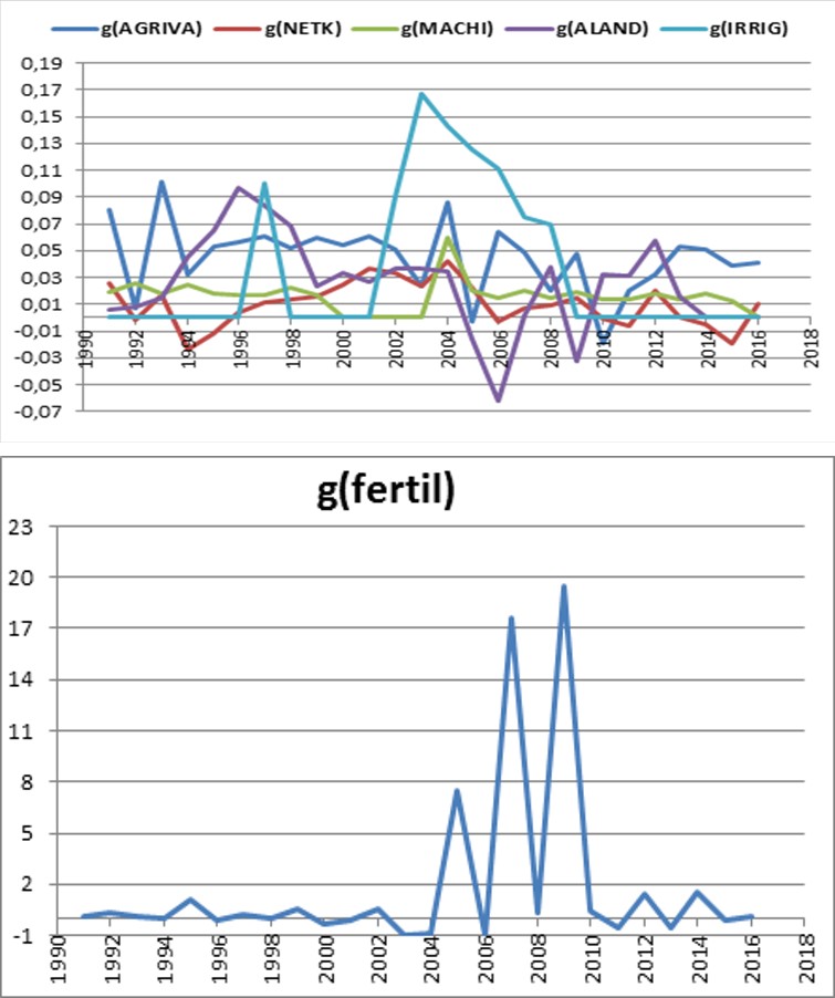
Figure 1a: Growth Rate of AGRIVA; NETK; MACHI; ALAND and; IRRIG.
Figure 1b: Growth Rate of FERTIL (1992-2018).
Linear Relationship between Agricultural Technologies and Agricultural Value-Added
Figure 2 explores the linear relationship between agricultural technologies and agricultural value-added over the period from 1992 to 2018. It reveals significant correlations between key technological factors and the growth of agricultural value-added. Mechanization and Agricultural Value-Added: In Figure 2a, the analysis demonstrates a strong positive correlation between the number of machines used in agriculture and agricultural value-added. This relationship suggests that increasing mechanization plays a vital role in enhancing agricultural productivity and, consequently, agricultural value-added. Irrigation Infrastructure and Agricultural Value-Added: Figure 2b examines the relationship between the area equipped for irrigation and agricultural value-added. It highlights a similarly strong positive correlation, indicating that improvements in irrigation infrastructure contribute significantly to the growth of agricultural value-added.
| Figure: 2(a) | Figure 2 (b) |
Figure 2(a) & Figure 2-(b): Relationship between Agricultural Value Added and Machinery and Area Equipped for Irrigation.
The findings imply that a linear model can effectively explain the relationship between these technological variables and agricultural value-added. Such models provide valuable insights for policymakers and stakeholders aiming to optimize agricultural production by leveraging mechanization and irrigation advancements.
Relationship between Chemical Fertilizers and Agricultural Value-Added: Figure 2c illustrates the relationship between chemical fertilizers and agricultural value-added over the period from 1992 to 2018. This figure examines whether there exists a linear association between the application of chemical fertilizers and the growth of agricultural value-added. The analysis reveals that the linear model has limitations in fully capturing the impact of chemical fertilizers, suggesting more complex interactions or nonlinear relationships.
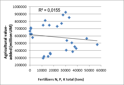
Figure 2c: Relationship between Agricultural Value Added and Fertilizers.
Limitations of Linear Models for Chemical Technologies: Figure 2c suggests limitations in linearly explaining the agricultural gross domestic product (GDP) based on the amount of chemical fertilizers used. This observation indicates that the impact of chemical technologies on agricultural value-added may involve more complex interactions or nonlinear relationships not captured by simple linear models. These relationships underscore the critical importance of mechanization and irrigation infrastructure in driving agricultural productivity and economic growth. They also highlight the need for nuanced approaches to understanding and utilizing chemical technologies to maximize their beneficial impact on agricultural production.
Impact of Chemical Fertilizers: The impact of chemical fertilizers on agricultural productivity and economic output shows a relatively weak linear relationship, with an R-squared value of 0.0155 and a p-value of 0.032. This indicates that other factors or more complex interactions likely influence the effectiveness of chemical fertilizers.
Relationship between Arable Land & Permanent Crops Area and Agricultural Value-Added: Figure 2d explores the relationship between the area dedicated to arable land and permanent crops and agricultural value-added from 1992 to 2018. This figure analyses the linear correlation between the expansion of cultivated land and the resulting increase in agricultural value-added. The results indicate a strong positive correlation, demonstrating that expanding arable land and permanent crop areas significantly enhances agricultural value-added.
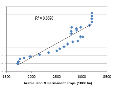
Figure 2d contributes to understanding the factors influencing agricultural value-added growth. Figure 2d: Arable Land and Permanent Crops.
Role of Expanding Arable Land and Permanent Crops Area: The role of expanding arable land and permanent crop areas in enhancing agricultural value-added is more significant, as evidenced by an R-squared value of 0.8598 and a p-value of 0.0021. This strong correlation underscores the importance of land expansion in driving agricultural growth.
These insights are crucial for developing strategies that optimize the use of chemical fertilizers and promote sustainable land use practices to foster long-term agricultural growth and economic stability.
Novelty of Analysis: The information in section 4.2 is novel for several reasons: 1. Empirical Evidence of Technological Impact Mechanization and Productivity: The section provides empirical evidence of a strong positive correlation between the number of machines used in agriculture and agricultural value-added. While the benefits of mechanization are known, this study quantifies the impact over an extended period (1992 to 2018), reinforcing the critical role of mechanization in agricultural productivity. Irrigation Infrastructure: Similarly, it highlights the significant positive correlation between the area equipped for irrigation and agricultural value-added. This empirical analysis underscores the importance of irrigation infrastructure, providing concrete data to support policy decisions. 2. Longitudinal Analysis: The analysis spans 27 years, offering a comprehensive view of the long-term trends and impacts of technological advancements on agricultural value-added. Many studies focus on shorter timeframes, but this extended period allows for more robust conclusions. 3. Linear Model Effectiveness Model Validation: The findings suggest that a linear model effectively explains the relationship between key technological factors (mechanization and irrigation) and agricultural value-added. This is significant because it provides a simple yet powerful tool for policymakers to predict and enhance agricultural productivity through technological investments. 4. Complexity in Chemical Fertilizer Impact Nonlinear Relationships: The section identifies limitations in using a linear model to explain the impact of chemical fertilizers on agricultural GDP. This observation is novel because it points to the need for more sophisticated models to capture the complex interactions of chemical inputs. This could lead to further research into nonlinear models or multi-factorial analyses to better understand the nuanced effects of chemical technologies.
Policy Implications
Actionable Insights: The findings offer actionable insights for policymakers and stakeholders. By highlighting the critical importance of mechanization and irrigation infrastructure, the study provides a clear direction for policy and investment priorities. It also suggests a need for nuanced approaches to chemical fertilizers, potentially leading to more targeted and effective agricultural policies.
Nuanced Technological Approaches
Chemical Technology Utilization: The section emphasizes the need for nuanced approaches to using chemical technologies. This is novel because it moves beyond the simplistic view that more chemical inputs always lead to higher productivity, suggesting instead that their impact may depend on other factors or conditions.
The novelty of the information in Section 4.2 lies in its empirical validation of the positive impacts of mechanization and irrigation on agricultural value-added, the identification of the limitations of linear models in explaining the impact of chemical fertilizers, and the provision of long-term data and actionable insights for policymakers. These contributions enhance the understanding of how different agricultural technologies affect economic outcomes and inform more effective strategies for optimizing agricultural production.
Empirical Results and Discussion
Unit-Root Test on Variables
To ensure the robustness of the data analysis, a logarithmic transformation was applied to the variables to stabilize exponential trends before conducting differencing. The results of the Augmented Dickey-Fuller (ADF) tests, presented in Table 3, indicate the presence of unit roots in the variables under consideration. (Appendix) -1 provides a note explaining the positive and negative values for the ADF test statistic and test critical values [28].
| Variables | Unit-root test in2 | ADF test statistic | Test critical values | Integration order |
|---|---|---|---|---|
| LAGRIVA | The first difference, including an intercept | -6.926025 | -3.724070*** | I(1) |
| LNETK | The first difference, without intercept or trend | -2.730906 | -2.660720*** | I(1) |
| LMACHI | The first difference, including an intercept | -4.06787 | -3.724070*** | I(1) |
| LCREDI | The first difference, without intercept or trend | -11.40214 | -2.664853*** | I(1) |
| LENERG | The first difference, without intercept or trend | -4.898979 | -2.660720** | I(1) |
| LLABOR | The first difference, including intercept and trend | -3.924902 | -3.673616** | I(1) |
| LALAND | The first difference, without intercept or trend | -2.077273 | -1.955020** | I(1) |
| LFORES | The first difference, including an intercept | -3.674498 | -2.986225** | I(1) |
| LIRRIG | The second difference is without intercept or trend | -5.234235 | -2.664853*** | I(2) |
| LFERTIL | The first difference, without intercept or trend | -6.700149 | -2.660720*** | I(1) |
Table 4: The Augmented Dickey-Fuller Unit-Root Test on Variables: Results.
*Indicates significance at the 1% level. Indicates significance at the 5% level. Source: Suitably developed programs in R-Language Table 3: The Augmented Dickey-Fuller Unit-Root Test on Variables: Results.
The null hypothesis of a unit root could not be rejected for the following variables even at the 1% significance level: agricultural value-added (LAGRIVA), net capital stock (LNETK), number of machines (LMACHI), amount of credit to agriculture (LCREDI), land equipped for irrigation (LIRRIG), and chemical fertilizer consumed (LFERTIL). However, the null hypothesis could not be rejected at the 5% significance level for the remaining exogenous variables. Subsequently, all variables were differenced to convert them into first differences or second differences in the case of land equipped for irrigation (LIRRIG) for further analysis. Differencing helps in removing the unit root and stabilizing the time series data, making it suitable for econometric modeling and analysis. This approach ensures that the empirical analysis is based on stationary time series data, facilitating accurate interpretation and reliable conclusions regarding the relationships and impacts of these variables on agricultural value-added growth in Bihar.
Estimation of Parameters αi
The growth of agricultural value-added was estimated using equation (4), and the results are summarized in Table 4. The econometric model employed includes an autoregressive component to capture the dynamics of agricultural value- added over time. Additionally, two dummy variables (Dum1, Dum2) were introduced to account for the influence of sectorial development policies and natural phenomena (e.g., flooding, precipitation) on agricultural value-added growth. The coefficients of these dummy variables were found to be statistically significant, rejecting the null hypothesis that their effects are equal to zero.
The regression model demonstrates robust performance, accurately predicting 99% of the specified equation. An F-statistic was computed to assess the overall significance and causality between the growth of agricultural value- added and its determinant factors.
Furthermore, diagnostic tests conducted on the residuals from the long-run model estimation—including tests for serial correlation, heteroscedasticity, and normality— indicate desirable properties. These tests ensure that the model assumptions are met, enhancing the reliability of the estimated parameters and the validity of the conclusions drawn regarding the factors influencing agricultural value- added growth in Bihar.
| Sample $ | ||
|---|---|---|
| Variable | Coefficient | S.E. |
| Constant | -103.5374** | 34.4886 |
| YEAR | 0.041686*** | 0.0119 |
| LNETK | 0.586066** | 0.20331 |
| LMACHI | 0.886031** | 0.35274 |
| LCREDI | 0.003155 | 0.00414 |
| LENERG | 0.958764 | 1.20027 |
| LLABOR | -0.029977 | 0.48857 |
| LALAND | 0.383954*** | 0.09456 |
| LFORES | 1.766482 | 1.25922 |
| LIRRIG | -0.268012*** | 0.08215 |
| LFERTIL | -0.004634* | 0.00242 |
| Dum1 | 0.079432*** | 0.01534 |
| Dum2 | -0.045332** | 0.0165 |
| AR(3) | -0.688183** | 0.27564 |
| Adjusted R2 | 0.997 | - |
| F-statistic | 800.48*** | - |
| Durbin-Watson stat (DW) | 2.358 | - |
Table 5: Estimation of the Growth of Agricultural Value-Added.
Sample$: 1990-2016 (N=27) *Indicates significance at the 1% level. Indicates significance at the 5% level. * Indicates significance at the 10% level. Source: Suitably developed programs in R-Language. Table 4: Estimation of the Growth of Agricultural Value-Added.
Prediction of the Growth of Agricultural Value- Added
This section evaluates the accuracy of the forecasted growth of agricultural value-added (LAGRIVAF) compared to the actual values estimated in section 5.2. The objective is to assess the adequacy of the estimated regression model in predicting agricultural value-added.
Forecasted Value Analysis: Figure 3a presents the forecasted values of LAGRIVAF, demonstrating a Root Mean Squared Error (RMSE) of only 1.146%. The curve of LAGRIVAF falls within the 95% confidence interval, indicating a high level of confidence in the forecast accuracy. The Theil Inequality Coefficient also suggests a close fit between the forecasted and actual values. Goodness of Fit Assessment: Based on these metrics, it can be concluded that the forecasted LAGRIVAF closely tracks the actual LAGRIVA values. The predictive power of the estimated regression model is deemed satisfactory, as depicted in Figure 3b where both LAGRIVA and LAGRIVAF are plotted together.
This analysis underscores the reliability of the regression model in predicting the growth trajectory of agricultural value-added in Bihar. The close alignment between forecasted and actual values enhances confidence in using the model for future projections and policy decisions aimed at fostering agricultural economic growth.
Forecast: LAGRIVAF Actual: LAGRIVA Forecast sample: 1990 2016 Adjusted sample: 1994 2016 Included observations: 23 Root Mean Squared Error 0.011460 Mean Absolute Error 0.008813 Mean Abs. Percent Error 0.065536 Theil Inequality Coefficient 0.000430 Bias Proportion 0.002990 Variance Proportion 0.009121 Covariance Proportion 0.987889 Figure 3a: Trend of Forecasted Growth of Agricultural Value-Added (1992-2018).
Figure 3b: Gap between Actual and Forecasted Growth of Agricultural Value-Added (1990-2016). Source: Suitably developed programs in R-Language.
Impulse Response of Agricultural Production Growth
This section examines how agricultural value-added in Bihar responds in the short, medium, and long terms to positive innovations or shocks in agricultural technology. The analysis employs Cholesky (d. f. Adjusted) innovation and was conducted using suitably developed R programming to model the impacts of various factors on agricultural value- added. The factors analysed include:
- Net Capital Stock (LNETK)
- Number of Machines (LMACHI)
- Number of Hectares of Arable Land and Permanent Crops (LALAND)
- Number of Hectares Equipped for Irrigation (LIRRIG)
- Number of Tons of Chemical Fertilizer (LFERTIL) Analysis and Graphical Presentation: The impulse response function (IRF) analysis was performed to determine how agricultural value-added reacts over different time horizons—short-term, medium-term, and long-term— to shocks in the aforementioned factors. The results are graphically presented and summarized in Table 5. Short-Term Response: In the short term, agricultural value- added shows a varied response to shocks in different factors. Initial reactions often include immediate positive or negative effects that stabilize over time as the system adjusts.
Medium-Term Response: Over the medium term, the response of agricultural value-added tends to reflect the adjustments and adaptations made in response to the initial shocks. For instance, capital investments and mechanization often show sustained positive impacts during this period, as the benefits of new technologies and infrastructure improvements are realized. Long-Term Response: In the long term, the impacts of the shocks become more evident. For some factors, such as net capital stock (LNETK), the initial positive response may diminish and turn negative if the capital is not renewed or reinforced. Conversely, innovations in machinery (LMACHI) and expansions in arable land and permanent crops (LALAND) typically continue to positively influence agricultural value-added growth.
The impulse response analysis highlights the following key points: Net Capital Stock (LNETK): Positive impact in the short and medium terms, with potential negative effects in the long term if not properly managed. Number of Machines (LMACHI): Consistent positive impact across all time horizons, emphasizing the importance of mechanization. Arable Land and Permanent Crops (LALAND): Steady positive influence, underlining the value of expanding cultivated areas. Irrigation (LIRRIG): Initial negative response that may reverse in the long term as proper irrigation management practices are adopted. Chemical Fertilizer (LFERTIL): Short-term negative response that transitions to a dominant positive effect in the long term, provided the balanced application is maintained.
The detailed response data is presented in Table 5, offering a comprehensive view of how agricultural value-added in Bihar reacts to technological shocks over different periods. In conclusion, the impulse response analysis underscores the need for strategic investment and management of agricultural technologies to sustain growth in agricultural value-added. By understanding these dynamics, policymakers can make informed decisions to enhance the resilience and productivity of Bihar’s agricultural sector.
| Period | LAGRIVA | LNETK | LMACHI | LALAND | LIRRIG | LFERTIL |
|---|---|---|---|---|---|---|
| 1 | 0.016548 | 0.000000 | 0.000000 | 0.000000 | 0.000000 | 0.000000 |
| 2 | 0.000938 | 0.001880 | 0.004575 | 0.003364 | 0.003025 | -0.006375 |
| 3 | 0.009523 | 0.000622 | 0.008313 | 0.003506 | -0.001925 | -3.58E-06 |
| 4 | 0.005766 | 0.001267 | 0.011745 | 0.010891 | -0.001772 | -0.002663 |
| 5 | 0.000604 | 0.003451 | 0.007465 | 0.016807 | -0.000977 | 0.003770 |
| 6 | 0.003461 | 0.005264 | 0.008238 | 0.018609 | -0.005930 | 0.002293 |
| 7 | 0.000132 | 0.003888 | 0.005086 | 0.016867 | -0.004091 | 0.001389 |
| 8 | 0.002821 | 0.002423 | 0.004726 | 0.012513 | -0.004422 | 0.001753 |
| 9 | 0.004001 | -5.71E-05 | 0.006643 | 0.009692 | -0.003263 | -0.000406 |
| 10 | 0.003092 | -0.001353 | 0.006889 | 0.009398 | -0.000784 | 0.001047 |
Table 6: Impulse Response of Agricultural Value-Added (1-10 Years).
Analysis of Agricultural Value-Added Growth in Bihar
Innovations in Machinery and Land Use: The recent advancements in machinery (LMACHI) and the expansion of arable land and permanent crops (LALAND) in Bihar have shown a consistently positive impact over the past ten years, as depicted in Figures 4c & 4d. These innovations appear to have a steady and favorable influence on the growth of agricultural value-added over a long-term period. Consequently, the pursuit of sustainable agriculture should focus on the adoption of mechanized technologies and farming practices that include multi-cropping and agroforestry.
Net Capital Stocks and Agricultural Growth: The growth of agricultural value-added in Bihar demonstrates a positive response to net capital stocks (LNETK) for the first eight years. However, this positive impact turns negative in the ninth and tenth years, as illustrated in Figure 4b. This pattern suggests that while capital investments positively affect agricultural value-added growth in the short and medium terms (1-8 years), their impact may diminish and become negative in the long term (after 8 years). Therefore, it is crucial to reinforce or renew capital investments at appropriate intervals to maintain a consistent positive trend in agricultural economic growth.
Irrigation Technologies: The response of agricultural value- added growth to a shock in irrigation technologies (LIRRIG) appears to be negative within the first ten years, as indicated in Figure 4e. However, this negative response may reverse after ten years. This reversal implies that once farmers adapt to soil characteristics and other factors related to irrigation management, these technologies could positively influence production growth.
Chemical Fertilizers: The positive response of agricultural value-added (LAGRIVA) to the impulse of chemical fertilizers (LFERTIL) tends to dominate the negative effects in the long term (after four years), despite the short-term negative impulse response, as shown in Figure 4f. For sustainable agricultural development, it is recommended that chemical fertilizers be applied in a balanced ratio. Overall Production System: Additionally, it has been observed that the output growth in Bihar reacts favorably within ten years when there is a direct shock to the overall production system, as depicted in Figure 4a. In summary, to achieve sustained growth in agricultural value-added in Bihar, it is essential to focus on:
- Continuing the adoption of innovative machinery and expanding arable and permanent crop areas.
- Reinforcing or renewing capital investments at opportune moments to sustain long-term growth.
- Appropriately managing irrigation technologies to eventually reverse any initial negative impacts.
- Applying chemical fertilizers in balanced ratios to mitigate short-term negative effects and enhance long- term positive impacts.
By implementing these strategies, Bihar can ensure a steady and sustainable growth trajectory in its agricultural sector.
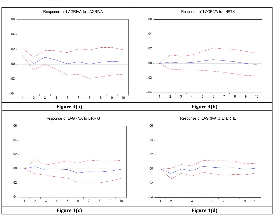
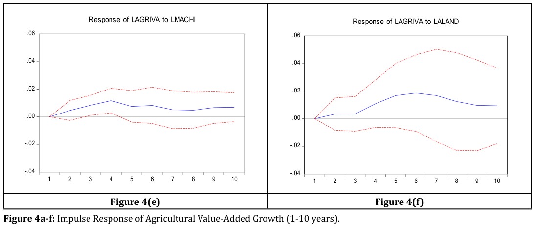
Figure 4a-f: Impulse Response of Agricultural Value-Added Growth (1-10 years).
Variations in Short-Term and Long-Term Results: A Comparative Analysis of Section 5.5 and Section 4.2: The variations between the results discussed in Section 5.5 and Section 4.2, particularly as depicted in Figures 2 & 4f, can be attributed to differences in methodologies, timeframes, and specific analytical focuses. These sections analyze the impact of various agricultural technologies on agricultural value- added in distinct contexts. Analytical Focus and Temporal Scope: Section 4.2 examines the long-term (1992-2018) linear relationships between specific agricultural technologies (machinery, irrigation) and agricultural value-added. It highlights strong positive correlations between the number of machines and irrigation infrastructure and agricultural value-added, suggesting these technologies have consistently positive impacts over the long term. Section 5.5: This section analyzes recent trends (past ten years) in Bihar’s agricultural sector, considering a wider range of factors impacting agricultural value-added, including machinery, capital stocks, irrigation technologies, chemical fertilizers, and overall production systems. It emphasizes specific short-term and long-term impacts that may vary across different technologies and timeframes. Timeframe and Specificity: Section 4.2: Focusing on a broader historical perspective (1992-2018), this section emphasizes long-term trends and linear relationships. It may not fully capture short-term fluctuations or recent developments observed in Section 5.5. Section 5.5: This section examines recent trends (last ten years), likely capturing more immediate effects and changes in response to newer technologies and economic conditions. Methodological Differences: Section 4.2: Utilizes linear modeling to establish relationships between technologies and agricultural value-added, assuming stable long-term effects reflected by linear correlations. Section 5.5: Employs a scenario-based analysis over a shorter period, which may reveal fluctuations and variable impacts that are not fully captured by long-term linear models. Complex Interactions and Nonlinear Relationships: Section 4.2: Suggest strong linear correlations for machinery and irrigation. Section 5.5: Introduces complexities such as diminishing returns for capital investments over time, initial negative impacts of irrigation technologies that later reverse, and mixed short-term and long-term effects of chemical fertilizers. These complexities imply that the impacts of technologies on agricultural value-added can be dynamic and context-dependent, varying over different time horizons and under changing agricultural practices. Integration and Understanding: Nuanced Approaches: While linear models provide valuable insights over long periods, they may oversimplify the dynamics observed in shorter-term analyses. Policy Implications: Policymakers should consider both long-term trends and recent developments to formulate robust strategies that account for both stable trends and emerging challenges in agricultural development. Further Research: Further research is needed to explore nonlinear relationships, time-varying effects, and the interactions between different agricultural technologies to inform sustainable agricultural policies and practices better.
By acknowledging these differences and integrating insights from both sections, stakeholders can develop more comprehensive approaches to enhance agricultural productivity and sustainability in Bihar and similar agricultural regions.
Agricultural Productivity & Income Growth
Enhancing agricultural productivity to augment farmers’ income remains a primary concern for policymakers. The analysis in previous sections underscores the significance of substantial investments in capital stock, specifically in mechanization, supported by infrastructure and timely adoption of new farming technologies. These measures are identified as crucial instruments for achieving the desired productivity and income growth.
The Special Task Force on Bihar (Government of India, 2008) echoed similar recommendations. It suggested financial outlays amounting to Rs 27055 crores for the period 2008-09 to 2012-13, in stark contrast to the Rs 1609 crores provisioned in the 11th Five Year Plan. Presently, the financial requirement for boosting agricultural productivity might constitute 1.5 – 2.0% of the Gross State Domestic Product (GSDP) for the Agriculture Sector.
The quantification of agricultural productivity and the resultant income for farmers is contingent upon the capacity of public expenditure. Additionally, the resultant crowding- in effect on private investment, along with various other systemic factors, plays a pivotal role in determining the outcomes.
In summary, strategic and substantial financial investment in agricultural mechanization, supported by robust infrastructure and timely adoption of innovative farming practices, is essential for boosting agricultural productivity and enhancing farmers’ income in Bihar.
Conclusions and Recommendations
This article examined the influence of agricultural technologies on the growth of agricultural value-added based on time series data (1992-2018) for Bihar. The following conclusions can be drawn from the study:
Conclusions
Technological Progress: Technological advancements have significantly enhanced the productivity potential of agricultural land in Bihar. Innovations such as multi- cropping, agroforestry, new seed varieties, and improved resource management practices have played a crucial role in boosting agricultural value-added growth. Capital Investment: Investment in capital stock has contributed 13% to the agricultural value-added. A 1% increase in capital stock results in a 0.59% increase in agricultural value-added, contingent upon the presence of adequate supporting infrastructure such as roads. Agricultural Mechanization: The adoption and utilization of agricultural machinery have accounted for 32% of the growth in agricultural value-added. This underscores the importance of mechanization in enhancing labor efficiency and reducing operational time. Short to Medium-Term Capital Stock Effects: The positive effects of net capital stocks on agricultural value-added are observed for the first eight years, but these effects turn negative in the ninth and tenth years. This indicates that while capital investments provide short to medium-term benefits, they may require reinforcement or renewal in the long term to sustain growth. Permanent Crops and Arable Land: Innovations in machinery and the expansion of arable and permanent crop areas have consistently contributed to agricultural value-added growth over ten years, demonstrating a steady positive impact. Permanent Cropping: Encouraging permanent cropping is advantageous, contributing approximately 21% to agricultural value-added in Bihar. Sustainable farming practices such as multi-cropping, crop rotation, and agroforestry positively influence growth, particularly for staple crops like rice, corn, and wheat. Irrigation and Fertilizers: Both the number of hectares equipped for irrigation and the use of chemical fertilizers exhibit a negative relationship with agricultural value-added growth. The potential negative externalities associated with these practices may outweigh their positive effects. Insignificant Variables: Variables such as labor, forest area, credit, and energy were not found to significantly impact agricultural value-added growth. This suggests that these factors do not directly contribute to increased agricultural value-added in the context of this study.
Recommendations
Large-Scale Capital Investment: Bihar should prioritize substantial investments in agricultural capital, given its significant impact on the growth of agricultural production value. Enhanced capital investment can drive productivity and economic gains in the agricultural sector. Timely Capital Renewal: It is essential to reinforce or renew capital investments at appropriate intervals to sustain a positive growth trend in agricultural economic performance. Periodic renewal ensures the continued efficacy of capital inputs over time. Mechanization and Labor: Increasing investment in agricultural mechanization can reduce labor requirements, enabling farmers to acquire new skills for operating advanced farming devices and implementing efficient resource management practices. Labor Force Enhancement: Strengthening the agricultural labor force with modern knowledge and practices is crucial. Training programs should focus on multi-cropping, agroforestry, the adoption of new seed varieties, and the expansion of arable and permanent crop areas, thereby positively impacting agricultural GDP growth. Credit Impact Analysis: The relationship between credit and agricultural value-added requires further investigation. This analysis should determine whether the current credit amounts are insufficient to generate meaningful returns or if there are issues related to credit management and utilization. Forests’ Environmental Role: Although the direct economic contribution of the forest sub-sector appears negligible, its environmental benefits, such as acting as carbon dioxide sinks, should be acknowledged and promoted. Emphasizing these positive externalities can enhance the environmental sustainability of agricultural practices.
To drive agricultural value-added growth in Bihar, sustained investment in agricultural technologies, timely reinforcement of capital stock, promotion of sustainable farming practices and enhanced mechanization are essential. Additionally, addressing the management and effectiveness of agricultural credit and recognizing the environmental benefits of forests will support sustainable agricultural development.
References
-
Hassanali A, Herren H, Khan ZR, Pickett JA, Woodcock CM (2008) Integrated pest management: the push- pull approach for controlling insect pests and weeds of cereals, and its potential for other agricultural systems including animal husbandry. Philosophical Transactions of the Royal Society B Biological Sciences 363(1491): 611.
-
Bale JS, Lenteren JCV, Bigler F (2008) Biological control and sustainable food production. Phil Trans R Soc B 363(1492): 761-776.
-
Goulding K, Jarvis S, Whitmore A (2008) Optimizing nutrient management for farm systems. Phil Trans R Soc B 363(1491): 667-680.
-
Roberts TL (2007) Fertilizer Best Management Practices: General Principles, Strategy their Adoption, and Voluntary Initiatives vs. Regulations. IFA International Workshop on Fertilizer Best Management Practice pp: 29-32.
-
David S, David Z (2000) The Agricultural Innovation Process: Research and Technology Adoption in a Changing Agricultural Sector. Handbook of Agricultural Economics pp: 103.
-
Nicholas K (1957) A Model of Economic Growth. The Economic Journal 67(268): 591-624_._
-
Wang KT, Zhou MJ (2006) An Analysis of Technological Progress Contribution to the Economic Growth in the Construction Industry of China. Construction & design for the project.
-
Solow RM (1956) A Contribution to the Theory of Economic Growth. Quarterly Journal of Economics 70(1): 65-94.
-
Sarel M Robinson DJ (1997) Growth and Productivity in ASEAN Countries. IMF Working Paper pp: 97/97.
-
Khan SU (2006) Macro Determinants of Total Factor Productivity in Pakistan. State Bank of Pakistan Research Bulletin 2(2): 384-401.
-
Patra S, Mishra P, Mahapatra SC, Mithun SK (2016) Modeling impacts of chemical fertilizer on agricultural production: a case study on Hooghly district, West Bengal, India. Model Earth System Environment 2: 180.
-
Kumar A, Yadav DS (2008) Long‐Term Effects of Fertilizers on the Soil Fertility and Productivity of a Rice- Wheat System. JACS 186(1): 47-57.
-
Weipeng C, Jian S (2013) Contribution of Agricultural Production Factors Inputs to Agricultural Economic Growth in Xinjiang. Guizhou Agricultural Sciences.
-
Sinha JK, Verma A (2017) Estimation of Capital Formation and Incremental Capital Output Ratio in Bihar (2004- 05 to 2011-12). The Journal of Income & Wealth 35(1).
-
Sinha JK, Verma A (2017) Trend and Growth of Capital Stock in Bihar. The Journal of Income & Wealth 35(2).
-
Sinha JK (2022) Public Expenditure for Agricultural Development & the Economic Growth of Bihar (1981- 2019). Asian Journal of Economics & Finance 4(4): 414- 424.
-
Sinha JK (2019) Influence of technologies on the growth rate of GDP from agriculture: A case study of sustaining economic growth of the agriculture sector in Bihar. Statistical Journal of the IAOS 35(2): 277-287.
-
Sinha JK, Sinha AK (2020) Trend and Growth of Capital Stock in Bihar During 1980-2017. Journal of Humanities Arts and Social Science 4(1): 57-66.
-
Sinha JK, Sinha AK (2022) Syndrome of Declining Economic Importance of Agriculture in Bihar (1960- 2018). Journal of Humanities Arts and Social Science 6(1): 1-15.
-
Dorward, A.et al. (2004) A policy agenda for pro-poor agricultural growth. World Development 32(1): 73-89.
-
Saha S (2012) Productivity and Openness in Indian Economy. Journal of Applied Economics and Business Research 2(2): 91-102.
-
Sivasubramonian S (2004) The Sources of Economic Growth in India, 1950-51 to 1999-2000. Oxford University Press, New Delhi, India, pp: 2(Y).
-
Viramani A (2004) Sources of India’s Economic Growth: trends in Total factor productivity.
-
Jingxian W, Yuyan Y (2011) Determining Contribution Rate of Agricultural Technology Progress with CD Production Functions. Energy Procedia 5(2011): 2346- 2351.
-
Zhao KJ (2011) Research on scientific and technological progress contribution to economic growth in Shandong Province. Journal of Shandong Jianzhu University.
-
Jinhe Z, Dengfeng C (2011) Estimating and forecasting the contribution rate of agricultural scientific and technological progress based on the Solow residual method. In“Proceedings of the 8th International Conference on Innovation & Management” pp: 281-287.
-
Annual Budget Documents for 2004-5 to2020-21, Finance Department, Govt. of Bihar, India.
-
Central Statistical Office, Govt. of India (2009) National Accounts Statistics: Sources & Methods.
- Enhancement of Vegetative Growth and Fruit Yield in Cucumber (Cucumis sativus L.) via Spiritual Blessing (Biofield) Energy Intervention
- Production of Açaí (Euterpe oleracea Mart.) under Different Agroforestry System Management Intensities in Amazonian Floodplain (Varzea) Forests
- Coffee and the Production Region: What is the Secret to the Expression "Quality"?
- Experiential Agripreneurship Training in Sub-Saharan Africa: Integrating a Business Incubator into Postgraduate Livestock Education at the University of Buea
- Advances in Agricultural High-Quality Development
- Linking Compost Residue to ABAGE in Plants - a Short Note