Steering Geometry of Remote Control Agricultural Vehicle
For any vehicle, steering mechanism is important one, in this research discuss importance of steering mechanism, what kind of steering mechanism used. For designing Unmanned remote control agricultural vehicle is rear wheel drive vehicle and front wheel is used for steer or turn the vehicle, but challenge for designing this type of vehicle is that unmanned remote control agricultural vehicle is not only working in flat road surface but it’s also used in agricultural field also. Another challenge was to working of steering system very fluently and reliable for farmer. The maximum steering effort was found 101.53 N for single wheel and angle for inner and outer wheel was 45.24° and 30.74° respectively. We have also found the turning radius of vehicle was 1490 mm.
Introduction
It’s challenging to design the steering system for an agricultural machine. Agricultural equipment is incredibly reliable, efficient, and ideal. The machine is more sensitive and has a better turning impact on the actual field [1]. Steering systems provide the necessary direction change. The primary challenge with the steering system is getting the vehicle to travel in an arc so that all four wheels revolve around the same centerline [2]. In order to maneuver a vehicle, the wheels must be turned, which requires a steering system. The wheels must constantly be in full rolling contact with the road. Sliding actions will wear out the tyres. When a vehicle is turning and all of the wheels form concentric circles, absolute rolling motion of the wheels on the road surface is possible. A vehicle’s directional response behavior is influenced by the steering system’s design. The purpose of the steering system is to provide the vehicle with overall directional control by steering the front wheels in response to driver inputs. The geometry of the suspension system, reactions, the geometry of the steering system, and the reactions of the powertrain, if the vehicle is front-wheel drive, all affect the actual steering angles.
To study the steering geometry firstly in 2011 Lili and co-workers tried to produce an Ackerman geometry system, but this process was limited to the calculation of the length of parts like the tie rod and it did not compare the performance [3]. Later in 2016 Malu and co-workers directly elaborated the effect of the steering moment arm angle and also used an iterative method for its prediction [4]. Then, in a study from Malik and co-workers from 2017 a discussion was carried out on suspension parameters that affect the steering characteristics but the limitation of this study was not discussing the steering parameters [5]. Then in the same year Biswal and co-workers designed the suspension parameters and steering types still this study lacked in the determination of the steering parameters [6]. Again, in the same year, Raut and co-workers threw light on energy transfer systems and suspension parameters and have not discussed the steering parameters [7]. Afterward, in 2018 Gitay and co-workers discussed the value of the parameters again, stating the iterative method for its vale prediction [8]. Lastly, in late 2018 Naveen and co-workers elaborated on the types of the steering system and the basis of its selection, but again a method for steering parameters goes missing [1]. So, from this, it was clear that a precise flow with the correct methods to find the steering parameters have always been missing, which is one of the main objectives of this paper. This research paper provides a step-by-step procedure on the decision and designing of steering parameters for a variable Ackerman geometry. It also includes a subtle overview of the selection of an appropriate steering mechanism. Firstly, a discussion is carried out on the methodology adopted for the designing of the steering mechanism. This includes the calculations for determining the Ackermann steering condition, turning radius estimation, space requirement calculation, trapezoidal steering system, design of variable Ackerman system, cross-checking steering effort value, minimizing bump steer, and getting the tie rod inboard point. Then the manufacturing of the steering mechanism is elaborated also its incorporation in the car is shown. Later the results obtained are discussed. Also, a stepwise method for the designing of the steering mechanism which was adapted in the manufacturing of our formula student car is explained. Additionally, a comparison of theoretical and analytical values is done. Lastly, a conclusion is made based on the study.
Ackerman systems are relatively differentiated based on the amount of tire scrub (i.e., produced by each mechanism while the car is taking a turn). There is no scrub in the Ackerman system; the scrub effect increases in parallel mechanisms and increases more in the anti-Ackerman systems. Also, the appropriate steering angle required for a turn is always a function of wheel load, road condition, turn speed (depends on turn radius), and tire characteristics. Since the car witnesses both high speed and low-speed corners, so there is no ideal steering mechanism possible unless controlling the steering angle for all the wheels is carried out independently [5].
The selection of Ackerman, Parallel, or Anti-Ackerman geometry depends on the vehicle’s cornering velocity during the turn. The cornering speed decides the amount of load transfer, further affecting the significance of slip angles on the car. As the slip angles have a higher impact at higher loads, it leads to the creation of lateral force accordingly [9]. The cornering velocity is directly proportional to the load transfer. Also, a slight difference in slip angles doesn’t create a significant impact on the performance (lateral force) of the car at similar loads. So, in low-speed corners, the Ackerman mechanism is preferred to prevent the momentum loss caused by the wheels’ scrubbing. Within the kinematic synthesis of a steering four-bar linkage, an input and an output link does not exist, but the two links must move in a coordinated fashion to comply with the steering condition. Under this condition, the two wheels carrying the links are required to move in such a way that the two axes of the wheels, OA and OB of Figure 1, intersect the rear axis OD of the vehicle. Therefore, although these two links remain close to parallel upon steering, their vertical axes rotate by differing angles. Although relatively small, this difference is significant enough to warrant careful consideration when designing the mechanism. Furthermore, a steering four-bar linkage is required to be symmetric for the vehicle to turn both right and left. Figure 2 shows the configuration of the wheels under a left turn. Based on the steering condition, the axes of the two wheels must intersect the rear axis at a common point O.
Materials and Methods
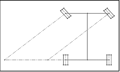
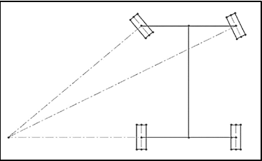
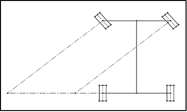
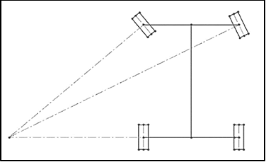
100% optimum steering arrangement is Ackermann because it prevents tyre slide at all four wheels. However, due to the slip angles created by the lateral force on the tyres, the effects of Ackermann steering diminish as the vehicle’s speed rises. The lateral force applied to a rubber tyre during a turn and the normal force on the tyre both have an impact on the slip angle of the tyre. It is, to put it simply, the angle formed between the tire’s alignment and its travel direction. . Slip angle occurs because rubber is a flexible material, thus as the bottom of the tire, the contact patch, is rolling along the ground at a velocity of 0, the rest of the tire causes the bottom material to lag behind for any given lateral force on the tire. This slip angle just slightly reduces the lateral force placed upon the wheel, and therefore the body of the car. The lateral force that is not caught in the spring action of the rubber tire then goes into turning the body [10]. Figure 3 shows a steering setup with parallel steering, while Figure 4 shows a steering setup with 100% Ackermann.
Condition for Perfect Steering
All four wheels must rotate at almost the same instantaneous centre in order for the steering to be perfect. The inner wheel negotiates a curve with a greater turning angle δi than the outer wheel’s axis δo, which is how vehicles navigate curves. Figure 1 demonstrates how a kinematic condition between the inner and outer wheels allows them to turn slip-free when the vehicle is travelling extremely slowly and turning to the left. This condition is called the Ackerman condition, which calculated by equation 1.
$$ \cot \delta o - \cot \delta i = \frac {w}{l} $$
(1) Where, δi is the steer angle of the inner wheel and δo is the steer angle of the outer wheel. The inner and outer wheels are defined based on the turning center o. The distance between the front and rear axles is called wheelbase, which is shown by ℓ. Additionally, the distance between the steer axes of the steerable wheels is called the track, which is shown by ω. Track ω and wheelbase ℓ are considered as kinematic width and length of the vehicle. The mass center of a steered vehicle will turn on a circle with radius R (Equation 2), $$ R = \sqrt {a _ {2} ^ {2} + l ^ {2} c o t ^ {2} \delta} \tag {2} $$ Where δ is the cot-average of the inner and outer steer angles, which computed by equation (3).
$$ \cot \delta = \frac {\cot \delta \mathrm {o} + \cot \delta \mathrm {i}}{2} \tag {3} $$ Angle δ is the equivalent steer angle of a vehicle with the same wheelbase ℓ and radius of rotation R.
In 2021, Vala and Yadav [11] said that proper design of agriculture implements is necessary to increase their working life and reduce the farming costs. In their study, Creo Parametric software was used to carry out finite element analysis of two components of remote control precision vehicle. 3D model of remote control precision vehicle was made using Creo 4.O software and static structural analysis were carried out using Creo 4.O simulation software.
Determination of Turning Radius
Turning radius was an important parameter of any self- propelled machinery like a tractor. Standard IS code [12] was referred for determination of turning radius.
Turning Diameter
Diameter of the circular path described by the centre of tyre contact with the surface of the test site of the wheel describes the largest circle when the developed vehicle is executing its sharpest possible turn under the test conditions [12].
Clearance Diameter
Diameter of the smallest circle, which will enclose the outermost points of projection of the developed vehicle and its equipment while executing its sharpest possible turn [12].
Testing Procedure for Determining Turning Radius (IS 11859:2004)
Drive the developed vehicle slowly forward while making its sharpest possible right-hand turn, that is, with the steering kept on full right-hand lock, at a speed not exceeding 2 km/h for at least one complete turn, until it is established that the minimum turning circle is being described. Continue to drive the developed vehicle slowly forward on the same lock for a further complete turn, at a speed not exceeding 2 km/h. At short regular intervals around the turn, mark on the ground those points coinciding with the centre of the tyre- to-ground contact area of the outermost wheel. Make the marks immediately behind this contact area and determine the position of each mark by visually projecting vertically downwards from the centre of the tyre tread width at points on the tyre circumference situated as close as possible to the ground.
Results and Discussion
Determination of Steering Effort
Steering effort was defined as the effort to be made by the driver (Linear DC actuator in our study) in turning the steering wheel. This could be calculated in either static condition i.e. when the vehicle was stationary and in dynamic conditions. Steering effort was maximum when the vehicle is stationary [13]. Force diagram on stationary wheel is shown in Figure 5.
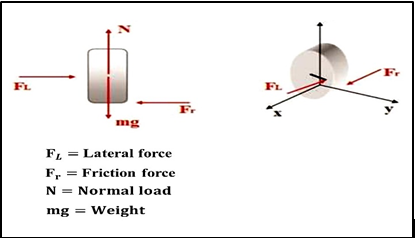
Mass of Vehicle = 131 kg Reaction weight on both front wheel = 34.5 kg Reaction weight on single tire = 34.5/2 = 17.25 kg Reaction on each front wheel = 17.25 × 9.81 = 169.22 N When the vehicle is stationary, the forces in all directions are in equilibrium (equation (4)).
$$ \begin{array}{l} \Delta F x = 0; F L = F R \tag {4} \\ \Delta F y = 0; N = m g \\ \end{array} $$ The tires used for the vehicle are barrow wheel and coefficient of friction between tires and ground was 0.6. The friction force at the tire is calculated by equation (5).
Friction force = μ × Reaction at each tire …(5) = 0.60 × 169.22 = 101.53 N for single wheel In the unmanned remote control agricultural vehicle most of all movement was controlled by remotely so for turning the vehicle DC linear actuator were used. Force developed by DC linear actuator be equal or greater than the frictional resistance of the ground to be able to turn the tire.
Steering Geometry
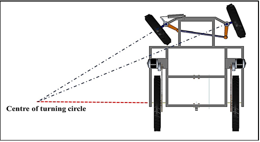
The Ackerman steering geometry was selected for the vehicle because this geometry enables the vehicle to turn about the common center i.e. without skidding of the tires and the Ackermann geometry is favored for the slow speed vehicle as the speed limit for the vehicle we are designing is 60 km per hour so it is the obvious choice. This geometry provides excellent control for low-speed maneuvering [12].
In Ackerman geometry the inside wheel turns more than the outside wheel. In this geometry, the rack was placed behind the front axle and if we extend the steering arms then they will meet at the extension of rear axle during turning, the point is the instantaneous center about which the whole vehicle turns without skidding, which is shown in Figure 6.
Reasons to Select Ackermann Type Steering System
- Reduce the weight of steering column or steering shaft because in Anti-Ackermann system the positioning of rack will be frontal portion of wheel centreline, which directly increases the shaft length.
- A parallel or reverse Ackermann system would be difficult to steer at low speeds, such as during a low speed run or moving the vehicle through the pits [9].
- Reverse Ackermann geometry is also difficult to achieve without longitudinal translation of the steering rack since the pickup points for the steering arms are on the outboard side of the kingpins. While this is possible to package at low steering angles, at higher steering angles collision becomes a major issue between the tie rod, upright, and wheel [9].
In order to properly validate and justify this, several cases taken into an account for the selection of perfect geometry [9]. So, we finally went in optimal to reduce the weight of the steering column and selected the Ackermann type steering system.
Inside and Outside Steering Angle
As the requirement, for our vehicle is to keep a turning radius minimum so it was decided that the outside turning radius of our vehicle should be minimum [13]. In unmanned remote control agricultural vehicle, turning radius was 1940 mm. Vehicle geometry was depicted in Figure 7 and turning radius can be calculated by equation (6). Where R is turning radius, b is wheel base, a is track width, c is width of frame and “∅” is outer wheel angle.
$$ R = \frac {b}{\sin \phi} + \frac {a - c}{2} \tag {6} $$
$$ 1 9 4 0 = \frac {9 4 0}{\sin \phi} + \frac {8 5 3 - 6 5 0}{2} $$
$$ 1 9 4 0 = \frac {9 4 0}{\sin \phi} + 1 0 1. 5 $$
$$ 1 8 3 8. 5 = \frac {9 4 0}{\sin \phi} + 1 0 1. 5 $$
$$ \sin \phi = \frac {9 4 0}{1 8 3 8 . 5} $$
sin = 0.51 φ
30.74 φ = °
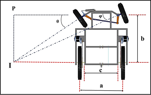
Now for correct steering geometry can calculate by using equation (7), where “θ” is inner wheel angle.
$$ \mathrm {e o t} \phi - \cot \frac {c}{b} \tag {7} $$
650 cot 30.74° - cot = 940 θ
1.68 - cot =0.69
$$ \begin{array}{l} 1. 6 8 - \cot \theta = 0. 6 9 \\ " \cot \theta = 0. 9 9 " \\ " \theta = 4 5. 2 4 ^ {\circ} " \\ \end{array} $$ Total steering angle =
$$ \theta + \phi = 3 0. 7 4 ^ {\circ} + 4 5. 2 4 ^ {\circ} = 7 5. 9 8 ^ {\circ} $$ For unmanned remote control agricultural vehicle at 1940 mm turning radius angle for inner and outer wheel was 45.24° and 30.74° respectively.
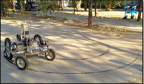
Turning radius of developed unmanned remote control agricultural vehicle was determined using a standard procedure (IS 11859:2004). Turing radius for the developed vehicle was 1490 mm (Figure 8).
Conclusion
This article proposed a steering mechanism that precisely satisfies the needs of unmanned agricultural vehicle and Ackermann turning geometry is best suited for our vehicle. In this article for unmanned agricultural vehicle design the Ackerman steering system and connect to DC linear actuator system. For that firstly determine steering effort for front wheel. Steering effort for steer the wheel was found 101.53 N for single wheel on that basis DC actuator was selected. For Ackerman steering mechanism we used DC actuator with 1500 N static load and 7 mm/sec actuating speed. For unmanned remote control agricultural vehicle at 1940 mm turning radius angle for inner and outer wheel was 45.24° and 30.74° respectively. Turing radius for the developed vehicle was 1490 mm.
Study Limitation
This study is related to only small scale unmanned agricultural vehicle and DC actuator with 1500 n static load for steering mechanism design for low speed of travel. DC actuator is 24 V DC power operated with 7 mm/sec linear speed of actuation.
Future Scope
According to this design, it is useful for designing big scale steering. Rather than using of fixed linear speed of actuation, in future study for variable speed actuation speed for different traveling speed and also check steer ability for different terrain.
References
-
Naveen J, Varma TD, Reddy S, Vardhan NG, Mouli KC (2018) Design of Steering Geometry for Formula Student Car’s. International Journal of Mechanical Engineering and Technology 9(5): 182-192.
-
de-Juan R, Sancibrian, Viadero F (2009) Optimal synthesis of Steering Mechanism Including transmission Angles. Proceedings of EUCOMES 08, pp: 175-181.
-
Lili D, Huaicheng X (2011) Optimization of race car divided steering trapezium. In 2011 International Conference on Electronics. Communications and Control (ICECC) IEEE, pp: 937-940.
-
Malu D, Katare N, Runwal S, Ladhe S (2016) Design methodology for steering system of an Atv. International Journal of Mechanical Engineering and Technology 7(5): 272-277.
-
Gautam P, Sahai S, Kelkar SS, Agrawal PS, Reddy DM (2021) Designing Variable Ackerman Steering Geometry for Formula Student Race Car. International Journal of Analytical, Experimental and Finite Element Analysis 8(1): 1-11.
-
Biswal S, Prasanth A, Udayakumar R, Sankaram MN, Patel D (2017) Design of steering system for a small Formula type vehicle using tire data and slip angles. MATEC Web of Conferences 124: 07007.
-
Raut C, Chettiar R, Shah N, Prasad C, Bhandarkar D (2017) Design, analysis and fabrication of steering system used in student formula car. Int J Res Appl Sci Eng Technol 5(5): 1529-1540.
-
Gitay NN, Joshi SA, Dumbre AA, Juvekar DC (2018) Design & Manufacturing of an Effective Steering System for a Formula Student Car. International Journal of Innovative Research in Technology 8(4).
-
Milliken WF, Milliken DL (1995) Racecar vehicle dynamics. Society of Automotive Engineers 400: 16-20.
-
McRae J, Potter JJ (2019) Design considerations of an FSAE steering system. Mechanical Engineering and Materials Sciences Independent Study, USA.
-
Vala VS, Yadav R (2022) Structural analysis of remote control precision planter using cad software. International Journal of Agricultural Sciences 18(2): 741-743.
-
IS 11859:2004 (2004) Guide for determination of turning radius and clearance radius. ISI, New Delhi, India.
-
Saini VK, Sunil KA, Shakya K, Mishra H (2017) Design methodology of steering system for all terrain vehicles. International Research Journal of Engineering and Technology 4(5): 454-460.
- The Expanding Landscape of Road Rage: A Systematic Review of Conflicts Involving Drivers, Pedestrians, and Micromobility
- Validating Cognitive Models of Royal Navy Performance on Control Systems
- Comparing Standard and State-of-the-art Firefighter Coats on Postural Balance and Gait in a Live Burn Environment
- Investigating the Integration of Telemedicine into Clinicians Workflow: A Review of Methods
- Risk Assessment of Ergonomic Factors in a Textile Firm by RULA, REBA and Fine Kinney Methods
- Impact of Self-Esteem Training on Individuals with Disabilities Aged 17-30