Optimizing a Variational Quantum Classifier through the Behavior Analysis of its Components
Quantum computer introduces a novel approach to process information. In quantum information processing, the law of quantum mechanics is applied to solve many practical computational problems. Classification is one such problem that can be resolved efficiently with the gate model quantum computer. There are several types of classifiers available in quantum domain, such as- variational quantum classifier (VQC), Quantum Support Vector Machine (QSVM) with Kernel Approximation, Hybrid Quantum Neural Network (QNN) etc. However, in this study, the mathematical similarities between VQC and classical support vector machine (SVM) and the components of the VQC are analyzed to optimize the performance of the classifier. For the convenience of the study, publicly available datasets, such as- IRIS dataset and Breast cancer dataset, are used in the experiments. IRIS dataset is brought into play for the testing and breast cancer dataset dimension reduced by Principle component analysis (PCA) is for validity test of the optimized VQC. After studying the VQC components in detail, it is found that the optimized VQC outperforms some of the classical machine learning algorithms or sometimes works as similar as classical SVM. The optimized VQC algorithm classifies IRIS dataset with 100% of accuracy and PCA dimension reduced Breast cancer dataset with 90% of accuracy. All of these studies are conducted with the help of Qiskit- an open-source software development kit (SKD) which is developed by IBM. So, the quantum device is considered to be ideal in every experiment.
Introduction
Quantum machine learning (QML) is an area of study where quantum computing and machine learning (ML) are intermingled to define and solve various real-life problems [1]. In quantum computing, computation is performed by utilizing the phenomenon of quantum mechanics [2].
Machine learning deals with the feature space of the empirical data to find generalized patterns and insights with the help of algorithms and statistical models without explicit instructions. In supervised machine learning settings, binary classifiers classify unknown data into two classes, y ∈ [−1, 1] based on what they learn from training instances {(x1, y1), (x2, y2),........,(xn, yn)}, where y ∈ [−1, 1] [3]. At first, the dataset of the problem is encoded in machines and is sent to the functions. The similarity is measured between the actual labels and the classified labels. Finally, the models are optimized by changing the hyper-parameters of the function that approximates the classes or labels. The linearly separable data is very straightforward and easy to classify. However, the real-life dataset, such as IRIS data sets, breast cancer data sets, Pandas datasets, etc., are not linearly separable. So, the kernel trick is applied to take the data to a higher dimensional feature space. But when feature space is getting larger, kernel function estimation becomes very expensive. Quantum computer offers a solution to this problem. With controllable quantum phenomena, there is a promise of achieving computational speed-ups through quantum algorithms [4]. Another phenomena is the similarity of the mathematical structure of the classical and quantum classifier. Moreover, the quantum feature map takes a feature vector to the Hilbert space automatically. So, kernel trick is unnecessary in quantum approaches. However, this is the Noisy Intermediate-Scale Quantum (NISQ) Technology era, where there are only less than 100 qubits in a quantum processor [5]. So, some scalable solutions are needed to be found for the current QML problems. Hence, hybrid quantum-classical architecture approaches are often taken to come up with solutions. One of the approaches contains a variational quantum circuit with a measurement operator and cost function. The variational quantum circuit are used to encode the data into the quantum circuit and tune the hyper-parameters with rotation gates, Rx, Ry and Rz [6, 7]. The cost function measures the similarity between the resultant label of the circuit and the actual label [8]. It also updates the parameters of the variational circuit. This process of updating the circuit hyper-parameters to train the circuit to recognize the correct label is often known as optimization. The optimization process of classifiers often gets stuck in local minima. The main goal is to avoid the local minima and to reach the global minima [8]. Only then the optimum hyper-parameters can be obtained for the quantum circuit. These optimal hyper-parameters ensure better solutions to the classification problems. With these ideas in mind, the experiments were conducted on the IRIS datasets. Some quantum classifier models are already proposed to address this classification problem. However, the training and testing accuracy were very poor and unstable. So, the circuit and the optimizer are not having the right hyper-parameters or the existing approaches get stuck in local minima. In this study, some experiments are performed to optimize VQC, and are tested on IRIS data set and breast cancer data set. The aim is to create an optimized quantum classifier that performs better or similar to the existing machine learning algorithm.
Mathematical Modeling of Classification Problem in Classical Setting
A dataset is given $\left\{ \begin{array}{l} \vec{x}_1, y_1, \vec{x}_2, y_2 \\ \dots \dots, \vec{x}_n, y_n \end{array} \right\}$ where $\vec{x}$ is a d-dimensional vector representing the numbers of features for algorithm and $y_i \in \{+1, -1\}$ for binary classification problem. $\vec{x}$ is another vector perpendicular to the decision line and $\vec{x}$ is a vector that shows a new data point. Now, to find out whether $\vec{x}$ is in the +ve or -ve side, $\vec{x}$
have to be projected onto $w$ to determine its location. If $\vec{x}+$ data points are for label, $y_i = +1$ and $\vec{x}-$ data points are for label, $y_i = -1$ and $b$ is a parameter, the equations for correctly classified data points are [16]:
$$\vec{w}.\vec{x}_+ + b \geq 1$$
$$\vec{w}.\vec{x}_- + b \leq 1$$
Now, for $y_i = (+1, -1)$, (1) and (2) equations can be rewritten as following [16]:
$$y_i(\vec{w}.\vec{x}_+ + b) - 1 = 0$$
where, the maximum width of the decision boundary is $\frac{2}{\|\vec{w}\|}$$
[16]. The support vectors lie at the edge of the boundary [17]. So, there are two constraints. One is equation (3) and another is the width of the boundary. If Lagrange multiplier is used, then the minimization of the result will be as below while honoring the both constraints. The primal form of the equation can be written as [18]:
$$L = \frac{1}{2} \| \vec{W} \|^2 - \sum_i \alpha_i [y_i(\vec{w}.\vec{x}_i + b) - 1]$$
Mathematical Modeling of Classification Problem in Quantum Setting
It is important to understand whether a VQC is mathematically or theoretically capable to solve any classification problem. In the classical machine learning setting, it has been seen that SVM is a linear classifier. Support vectors helps to determine that boundary between two classes. According to the equation (4), classification issues are just convex optimization problems which can be solved effectively with classical machines. But in this study, quantum algorithm is to be implemented to check whether the algorithm performs better than classical ones or any quantum advantage can be achieved. In this section, the theoretical analysis of the classification problem is discussed and it is shown that VQC is also a linear classifier like SVM. In the procedure, at first the dataset is needed to take data points to the higher dimensional vector space, $\emptyset : x \rightarrow \phi(z)$ where, $\emptyset$ is non-linear [19]. Then, the dataset is linearly classified. To ensure this, the following equation is to be found out [19]:
$$f_\theta(z) = \langle \phi(z) \mid w_\theta^+ ZW_\theta \mid \phi(z) \rangle \in [-1, +1]$$
At first, consider that [19], $H_\theta = W_\theta^+ ZW_\theta$ (6)
Where, $H_\theta$ is optimized over the Hamiltonian or the observable against the feature vectors. Now,
$$f_\theta(z) = \langle \phi(z) \mid H_\theta \mid \phi(z) \rangle$$ (7)
$< \phi(z) \mid H_\theta \mid \phi(z)$ is a 1-dimensional scalar number whose trace is equal to the number, itself.
$$f_\theta(z) = \text{Tr} \left[ \langle \phi(z) \mid H_\theta \mid \phi(z) \rangle \right]$$ (8)
So, $f_\theta(z) = \text{Tr} \left[ \langle \phi(z) \mid H_\theta \mid \phi(z) \rangle \right]$ (9)
It is also known that, $\|\phi(z)\| > \|\phi(z)\|$ is a density matrix in $2^n \times 2^n$ complex vector space which is another representation of $\phi(z)$ or mathematically,
$$\phi(z) \approx \|\phi(z)\| < \phi(z)$$ (10)
$$f_\theta(z) = \text{Tr} \left[ H_\theta \phi(z) \right]$$ (11)
If $H_\theta$ and $\phi(z)$ can be decomposed as following [19]:
$$H_\theta = \frac{1}{(2)^n} \sum_{\alpha \in 4^n} < H_\theta P_\alpha > P_\alpha$$ (12)
$$H_\theta = \frac{1}{(2)^n} \sum_{\alpha \in 4^n} \text{Tr} \left[ H_\theta P_\alpha \right] P_\alpha$$ (13)
Let, $h_\alpha(\theta) = \text{Tr} \left[ H_\theta P_\alpha \right]$ (14)
So, it can be written, $H_\theta = \frac{1}{(2)^n} \sum_{\alpha \in 4^n} h_\alpha(\theta) P_\alpha$ (15)
Similarly, $\phi(z) = \frac{1}{(2)^n} \sum_{\alpha \in 4^n} < \phi(z), P_\alpha > P_\alpha$ (16)
which can be written as [19]:
$$\phi(z) = \frac{1}{(2)^n} \sum_{\alpha \in 4^n} \phi(z) P_\alpha$$ (17)
So, equation (11) can be rewritten as following [19]:
$$f_\theta(Z) = \text{Tr} \left[ \left( \frac{1}{(2)^n} \sum_{\alpha \in 4^n} h_\alpha(\theta) P_\alpha \right) \left( \frac{1}{(2)^n} \sum_{\alpha \in 4^n} \phi(Z) P_\alpha \right) \right]$$ (18)
This can be combined and written as [19]:
$$f_\theta(Z) = \frac{1}{(4)^n} \text{Tr} \left[ \left( \sum_{\alpha \in 4^n} h_\alpha(\theta) \phi(Z) P_\alpha \right) \right]$$ (19)
$$ f _ {\theta} (Z) = \frac {1}{(4) ^ {n}} \sum_ {\alpha , \beta \in_ {4} ^ {n}} h _ {\alpha} (\theta) \phi (Z) \operatorname {T r} \left[ P _ {\alpha} P _ {\beta} \right] $$ Or, (20) It is known that [19], $$ \operatorname {T r} \left[ \mathrm {P} _ {\alpha} \mathrm {P} _ {\beta} \right] = 2 ^ {\mathrm {n}} \mathrm {i f} \alpha = \beta \mathrm {a n d} 0 \mathrm {i f} \alpha \neq \beta $$ (21) $$ \mathrm {f} _ {\theta} (Z) = \frac {1}{(2) ^ {n}} \sum_ {\alpha \in 4 ^ {n}} \mathrm {h} _ {\alpha} (\theta) \phi (Z) $$ So, (22) $$ f _ {\theta} (Z) \in [ - 1, + 1 ] $$ This (23) If threshold, [ ] b 1,1 ∈− , [ ] b 1, 1 ∈−+ +then, it can be written [19], ( ) 4 1 ( ) ( ) (2) $$ \operatorname {l a b e l} (Z) = \operatorname {s i g n} \left(\frac {1}{(2) ^ {n}} \sum_ {\alpha \in 4 ^ {n}} h _ {\alpha} (\theta) \phi (Z) + b\right) \tag {24} $$ which is equal to the solution, $$ \operatorname {L a b e l} (Z) = \operatorname {s i g n} \left(f _ {\theta} (Z) + b\right) \tag {25} $$ $$ x \approx f _ {\theta} (z), $$
, as x data point is mapped to
( ) f z θ , so, † ( ) ( ) Label Z
sign w x
$$ 0 = \operatorname {s i g n} \left(w ^ {\dagger} x + b\right) \tag {26} $$ Now, the primal form of the equation can easily be worked out just like classical SVM algorithm as from equation (3) and (4) by solving for the optimal separating hyper plane given as following:
( )
| 1 | w |
|---|---|
| 2 |
(27)
Classification with Variational Quantum Classifier Model
At first, the unitary gates ( ) U θ are applied to the initial states of the quantum circuit, | 0 n > in a quantum variation classifier (VQC). The parameters of ( ) U θ depend on the dataset of the problem. A variational circuit block ( ) W θ is added. This block is tuned, tested and optimized. After that, the circuit is measured on Z-basis. The result is a string of bit, { } 0,1 n z ∈ . Then, the string of bits is mapped to a cost function, C. The actual labels are compared with the labels from the circuit. After that, optimizer is used to optimize the circuit. The optimizer feed ( ) W θ with a new set of parameters. The circuit is rerun and from that the expectation value, ( ) ( ) ( ) ( ) † z z p x W M W x ϕ θ θ ϕ = ρ ρ ρ ρ is estimated. These values are again mapped to { } 1, 1 C ∈+ − [20]. The circuit is rerun again and again until the optimum hyper parameters are reached. This algorithm is applied on the test data to check the performance of the algorithm. This time the parameters of ( ) W θ are fixed.
In classical ML algorithm, the dataset, X, is imported into a ML model. The model takes the data and provides a prediction or answer. The model depends on the parameter, θ . Then there is a cost function which compares the performance of the model with actual answer. The optimizer optimizes the algorithm performance by updating the parameter of the ML model. The model is then applied to test dataset to check the performance of the algorithm. In QML, the classical ML model portion is replaced by a quantum circuit. This circuit consists of encoding and parameterized circuit. The measurement operator in the architecture is to obtain the output of the circuit. Before training a quantum circuit, the classical data are needed to be encoded into the quantum states. To do that, the unitary transformation gates are used. So, the raw data, d x ∈ ρ is mapped to a new quantum state, ( ) ( ) ( ) 2 n x x φ φ ⊗ >< ρ ρ Σ ò [21]. In this state, dimension of all linearly inseparable data is increased and mapped to higher dimensional Hilbert space. A variational quantum circuit is added to the new quantum state, ( ) ( ) ( ) 2 n x x φ φ ⊗ >< ρ ρ Σ ò [21]. This variational circuit depends on the parameter, θ . After that, the circuit measurement is performed on Z-basis and $$ \left(z\right) \epsilon \left\{- 1, + 1 \right\} $$ is calculated. [21] This is the result of
labeling bit string
{ } 0,1 n z ∈
based on the Boolean function
$$ f: \{0, 1 \} ^ {n} \rightarrow \{+ 1, - 1 \}, \mathrm {S o}, \mathrm {i f} $$ $$ f (z) \epsilon \{- 1, + 1 \} $$ is the label of the dataset, then probability of measuring one or another label is[4]:
$$ p _ {y} = \frac {1}{2} (1 + f (z) (< \varphi (\vec {x}) \left| W ^ {\dagger} (\vec {\theta}) f W (\vec {\theta}) \right| \varphi (\vec {x}) > $$ where, $$ f = \sum_ {z \in \{0, 1 \} ^ {n}} f (z) | z > < z | \tag {28} $$ The circuit diagram of this VQC model is shown below Figure 1:
![Figure 1: Architecture of VQC [20].](/fulltextimages/9155/fig_1.png)
The equation (28) is needed to be solved and it is
required to answer what is
$$ p _ {z} \mathrm {a n d i f} p _ {z} \mathrm {i s} \mathrm {p} _ {+ 1} \mathrm {o r}, p _ {- 1}. \mathrm {T h e} $$
result is compared with the actual label to determine the
performance of the quantum model.
A threshold has to be defined after that. Various optimization techniques are used to update the parameters of VQC model. These updated parameters are fed to the ( ) W θ block and are tuned and tested as long as optimum θ values for the classifier are not found. However, the values of θ are also depended on the unitary gates in the circuit. As Hilbert space is a complex vector space, some parameters of ( ) W θ is not accessible by quantum gate operation [22]. So, only the subset of those parameters can only be accessible to optimize the equation. It is also import to remember that the more parameter the circuit can access, the better the expressivity of the quantum circuit [23, 24]. But better expressivity does not mean that the circuit is going to be performing better in classification or any machine learning problem [8]. Moreover, it can be seen that the computation is basically done by quantum circuit. Cost analysis and optimization are done by classical machines. So, the quantum classifier is like a hybrid loop. This loop optimizes the circuit performance.
Components of Variational Quantum Classifier
Variational quantum classifiers have several essential components. In this experiment, only three of them are analyzed. They are:
- Encoder,
- Ansatz circuit and
- Optimizer
Encoder circuit
Encoder circuit is a kind of circuit that prepares quantum states according to the feature values of a data point [8]. The experiments are run with three types of encoders. They are PauliFeatureMap circuit, Z Feature map circuit or one form of angel encoding and ZZ FeatureMap circuit or higher order embedding [25]. 1. PauliFeature Map circuit: Pauli matrices are I, X, Y and Z matrices. The Pauli variables contain these quantum gates. This kind of feature mapping transfers the raw data, d x ∈ ρ to $$ \bar {x} \in \mathcal {R} ^ {d} \mathrm {t o} U _ {\varphi (\bar {x})} = \exp \left(i \sum_ {\mathrm {S} \subseteq [ \mathrm {n} ]} \varphi_ {\mathrm {s}} \left(\bar {\mathrm {x}}\right) \Pi_ {\mathrm {i} \in \mathrm {S}} \mathrm {P} _ {\mathrm {i}}\right) $$ , where S describes the connection between data points [25]. This circuit can be repeated in operation. For Pauli string P0=Z and P0,1=ZZ (k=2) and P0=Z(k=1), the Pauli Feature Map circuit can be drawn as below Figure 2.
$$ \begin{array}{l} q _ {0}: H \\ q _ {1}: H X U 1 (2. 0 * (\pi i - x [ 0 ]) ^ {*} (\pi i - x [ 1 ])) X \\ \end{array} $$ Figure 2: Example of Pauli Feature Map circuit [25].
2. Z Feature Map: Z Feature map is the first order Pauli-Z evolution circuit [25]. It is a sub-class of Pauli feature map [25]. The input data is needed to be fed to the customized U1 gates. In the figure below, a 3-qubit Z feature map circuit is illustrated in Figure 3.
3. ZZ Feature Map: ZZ Feature Mapping is an example of higher order feature mapping circuit. It is the second order Pauli-Z evolution circuit [25]. To employ this feature mapping model, the features of the data are required to be encoded in the qubit and the values of the U1 gates are assigned for each qubit. A two qubit, single repetition ZZ Feature Map circuit is shown in the Figure 4 below:
$$ \begin{array}{l} q _ {0}: H U 1 (2. 0 * x [ 0 ]) \\ q _ {1}: H U 1 (2. 0 * x [ 1 ]) X U 1 (2. 0 * (\pi - x [ 0 ]) ^ {*} (\pi - x [ 1 ])) X \\ \end{array} $$ Figure 4: Two-qubit ZZ Feature map circuit [25].
Ansatz Circuit
The Ansatz or parameterized circuit is one of the essential parts of the variational quantum classifiers. It comprises of rotation gates and CNOT gates. The rotation gates are used to tune and to adjust the hyper parameters of the quantum circuit and to improve the classifier performance. When the optimum hyper parameters are found from the optimizer, those parameters are fed to the quantum circuit. CNOT gates ensure entanglement between the encoded data. This entangling layer is used to ensure that the states of the qubits can get interacted and the quantum computational advantage can be achieved. Moreover, simulating entangled qubit or ansatz is a hard task for classical computers. An example of a parameterized circuit is illustrated in the figure 5 below. This ansatz has been implemented in this study.
$$ \begin{array}{l} q _ {0}: \mathrm {R Y} (\theta [ 0 ]) \\ q _ {1}: \mathrm {R Y} (\theta [ 1 ]) \quad X \\ q _ {2}: \mathrm {R Y} (\theta [ 2 ]) \quad X \quad X \quad \mathrm {R Y} (\theta [ 5 ]) \\ \end{array} $$ Figure 5: Architecture of Ansatz circuit [25].
Optimizer
Optimization is the process in which the differences between predicted label and target label are studied. The hyper parameter of the VQC circuit is tuned and the loss function is tried to reduce to find an optimum boundary between two classes. In VQC, classical computers are used to optimize the performance of a quantum classifier. The hyper parameter for the optimizer are fed to the circuit and the hybrid loop continues in the process of optimization.
Five different types of optimizers are elaborately analyzed in this study. They are Adam and AMSGRAD optimizers (ADAM), Analytic Quantum Gradient Descent (AQGD) with Epochs optimizer, Constrained Optimization By Linear Approximation optimizer (COBYLA), Sequential Least SQuares Programming optimizer (SLSQP) and Truncated Newton (TNC) optimizer [25].
Experimental Analysis and Results
As discussed earlier, the quantum classifier is a linear classifier. However, VQC classifier cannot classify more than two labels at a time. So, only two classes were extracted out from the given dataset at first. There are other approaches in QML which may have the chance to classify more than 2 classes at a time. In Figure 6, sample images of IRIS dataset are shown:
At first the structure of the problem is analyzed by visualizing the given data. In the Figures 7 and 8, IRIS dataset is plotted which contains three classes based on the patel length and patel width. In this setting, setosa and versicolor can be easily separated with linear boundary but it is hard to classify versicolor and virginica linearly.
![Figure 3: Figure 3: Three-qubit Z feature map circuit [25].](/fulltextimages/9155/fig_3.png)
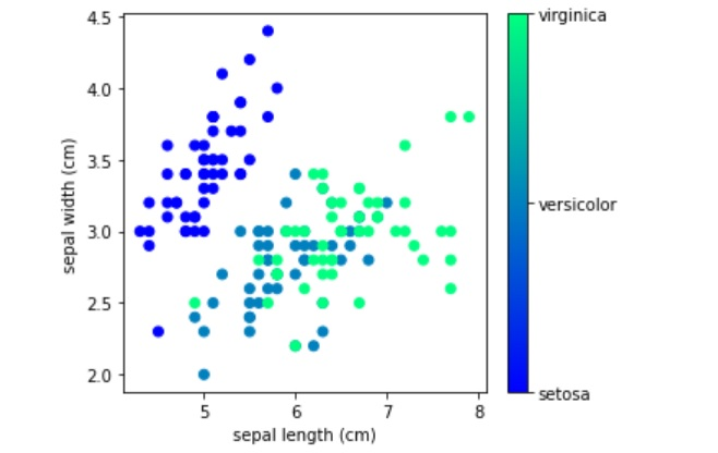
Now, the pattern of data has to be checked based on the other two properties of IRIS dataset. They are- sepal length and sepal width. Here, it can be seen that virginica and setosa can be easily classified but it is hard to classify versicolor and virginica. Figure 8 shows the distribution of the three classes based on these two properties of IRIS dataset.
![Figure 4: Two-qubit ZZ Feature map circuit [25].](/fulltextimages/9155/fig_4.png)
It can be understood from Figures 7 and 8 that there are four properties or features of each data. If VQC algorithm should be run on this dataset, it should be ensured that the qubit states alter with the values of the features of each data point [8]. As the data is four dimensional, four quantum bits are required [8]. The test dataset sample of IRIS dataset is shown in Figure 9 below:
![Figure 5: Architecture of Ansatz circuit [25].](/fulltextimages/9155/fig_5.png)
Encoder Circuit Analysis
The most significant part of QML algorithm is the encoder circuit. In many of the cases the encoder circuit determines how the algorithm will perform. So, it is really necessary to choose right encoder with correct depth to solve classification problem with quantum computers. From the discussion of the feature map circuit, it can be found out that all the feature mapping circuits, such as- Pauli Feature map, Z Feature map and ZZ Feature map, start with H operation. After that, the rotation operations are applied as per values of the data.
These three types of feature mapping circuit are experimented along with five types of optimizers. The parameterized circuit remains the same. The results are shown below as in the Table 1,
| Encoding Circuit | Performance on Test Dataset | ||||
|---|---|---|---|---|---|
| ADAM | AQGD | COBYLA | SLSQP | TNC | |
| PauliFeatureMap | 70% | 70% | 75% | 80% | 80% |
| ZFeatureMap | 95% | 70% | 100% | 100% | 100% |
| ZZFeatureMap | 70% | 70% | 75% | 80% | 80% |
Table 2: Performance of Different Encoding Circuit.
From the table 1, it can clearly be said that Z feature map has performed better than all the other types of circuit and the classifier has the similar results from PauliFeature map and ZZFeature map circuits.
With ADAM optimizer, it can be seen that only Z feature map reaches 95% accuracy where as other feature maps remain as 70% of accuracy. If AQGD optimizer is in operation, the feature map circuits have no impact on the overall performance of the algorithm. Again, with Z feature map and COBYLA optimizer, the accuracy result is 100% and other feature maps have got 75% accuracy. SLSQP and TNC optimizers have performed the same. In these cases, Z feature map is appeared to be the best option.
| Encoding Circuit Depth | Performance on Test Dataset | ||||
|---|---|---|---|---|---|
| ADAM | AQGD | COBYLA | SLSQP | TNC | |
| 1 | 95% | 70% | 100% | 100% | 100% |
| 2 | 75% | 90% | 100% | 100% | 100% |
| 3 | 70% | 80% | 75% | 80% | 85% |
Table 3: ZFeature Map Encoder Performance.
From the Table 2, it can be understood that when Z Feature map is implemented with circuit depth 1 and 2, the accuracy is 100% with COBYLA, SLSQP and TNC optimizer. Up until now, three optimizer works with high accuracy when the dataset is lower dimensional (In this case, dimension of data =4) by using Z feature map and circuit depth is 1 and 2. But encoder depth 1 does not always provide good results. All in all, when there is a quantum circuit with depth 2, then this configuration have the best possible results for almost all classifiers. The performance analysis of the encoder circuit (Z Feature Map, Depth=2) is illustrated in table 2. It can be seen that overall depth 2 circuit provides the best results. Anstaz Circuit Analysis Ansatz is one of the major components of VQC. It is very important to choose right ansatz and its depth to solve any classification problem. In this study, the ansatz shown in figure 5 is used. The circuit depth is changed to check the overall performance of the classifier. The Pauli Feature Map is not mentioned here, because it works as similar as ZZ feature map in the experiments. The detail analysis of VQC performance is shown in the bar chart below (Figure 10).
![Figure 6: Sample images of IRIS dataset [26].](/fulltextimages/9155/fig_6.png)
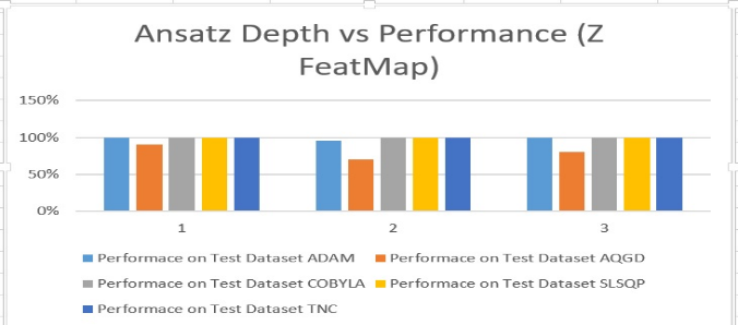
In figure 10, performance analyses of the bar diagram of VQC (ZZ Feature map and Ansatz depth 2) are illustrated. In this setting SLSQP and TNC perform better than all the other combination. The classification accuracy is 80% in these settings. When ansatz depth is 2, lesser resources are needed to build that quantum circuit. However, one might think that more circuit depth makes more parameter shift. Hence, it is probable to get better result if the circuit depth is increased. However, more parameter does not necessarily ensure better performance of Ansatz in the operation of VQC. Figure 10 and 11 demonstrates this clearly. But two optimizers, SLSQP and TNC always perform very well with any kind of circuit depth. However, TNC is always working better than SLSQP. This will be shown in validity test. With Z feature map (depth 2), the ansatz (depth=2) and TNC optimizer, the optimum parameters of the ansatz of this classification problem are: opt_params [6.47534855 -1.11200387 3.34001454 5.37309336 2.57341714 3.70006039 5.29063351 -0.27497174 5.58621329 2.66845098 4.9311402
4.31889917 4.76254717 4.40608396 4.81049839 0.03453597]
Optimizers Performance Analysis
In this study, five types of optimizers are used. They are- ADAM, AQGD, COBYLA, SLSQP and TNC. Here, their performance will be analyzed. The encoder, the depth of encoder, ansatz and its depth, are chosen already. Now, it is time to identify the efficient optimizer. All this optimizer is tried out one after another and the cost function are analyzed. It is important to note that the attempt is to reduce the cost function in the classical or quantum machine learning algorithm.
It is also important to check how optimizers perform in different circuit settings. So, at first, VQC settings are tested with ZZ feature map and ansatz circuit and their depth 1. The result of the classifier performance is shown in the Figure 12.
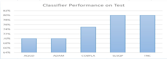
The Figure 12 shows that AQGD and ADAM optimizers obtain 70% of accuracy; COBYLA’s accuracy is 75% whereas SLSQP and TNC are having 80% classification accuracy. So, from another experiments as shown in figure 13, it can be determined that SLSQP and TNC work better. So, that optimizer can be applied in the algorithm to get the optimum performance from the classifier.
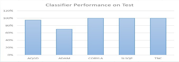
In this study, it can be seen that ADAM optimizer’s performance is the lowest. It is about 70%. AQGD has got 95% accuracy. However, as it is expected that COBYLA, SLSQP and TNC have performed better. They could classify the dataset with 100% of accuracy. The optimum value obtained from the cost function is- opt_value 0.010566505534852494 However, it is needed to be ensured that the classifier works similarly in other datasets. Hence, in the following part, the validity of this result will be checked to understand the best arrangement of the VQC algorithm.
Results of this Classification Problem
The results below shows actual label and probabilities of getting a certain label. If the probability of a label is more than 0.5, the classifier assigns that label to the respective data point. Data point:[6. 2.7 5.1 1.6] Actual: versicolor, Probabilities [{‘setosa’: 0.20542, ‘versicolor’: 0.79458}] ---------------------------------- Data point:[5.5 2.3 4. 1.3] Actual: versicolor, Probabilities [{‘setosa’: 0.20327, ‘versicolor’: 0.79673}] ---------------------------------- Data point:[5.9 3.2 4.8 1.8] Actual: versicolor, Probabilities [{‘setosa’: 0.25627, ‘versicolor’: 0.74373}] ---------------------------------- Data point:[4.8 3. 1.4 0.3] Actual: setosa, Probabilities [{‘setosa’: 0.80014, ‘versicolor’: 0.19986}] ---------------------------------- Data point:[5.1 3.8 1.9 0.4] Actual: setosa, Probabilities [{‘setosa’: 0.69402, ‘versicolor’: 0.30598}] ---------------------------------- Data point:[5.1 3.4 1.5 0.2] Actual: setosa, Probabilities [{‘setosa’: 0.79133, ‘versicolor’: 0.20867}] ---------------------------------- Data point:[4.6 3.6 1. 0.2] Actual: setosa, Probabilities [{‘setosa’: 0.61392, ‘versicolor’: 0.38608}] ----------------------------------
Data point:[5.5 2.4 3.8 1.1] Actual: versicolor, Probabilities [{‘setosa’: 0.21275, ‘versicolor’: 0.78725}] ---------------------------------- Data point:[5.4 3.7 1.5 0.2] Actual: setosa, Probabilities [{‘setosa’: 0.90318 ‘versicolor’: 0.096818}] ---------------------------------- Data point:[5.1 3.5 1.4 0.2] Actual: setosa, Probabilities [{‘setosa’: 0.78484, ‘versicolor’: 0.21516}] ---------------------------------- Data point:[5.7 3.8 1.7 0.3] Actual: setosa, Probabilities [{‘setosa’: 0.75274, ‘versicolor’: 0.24726}] ---------------------------------- Data point:[4.8 3.1 1.6 0.2] Actual: setosa, Probabilities [{‘setosa’: 0.78109, ‘versicolor’: 0.21891}] ---------------------------------- Data point:[6.1 2.8 4.7 1.2] Actual: versicolor, Probabilities [{‘setosa’: 0.24934, ‘versicolor’: 0.75066}] ---------------------------------- Data point:[5.5 4.2 1.4 0.2] Actual: setosa, Probabilities [{‘setosa’: 0.78450, ‘versicolor’: 0.21550}] ---------------------------------- Data point:[5.5 2.6 4.4 1.2] Actual: versicolor, Probabilities [{‘setosa’: 0.17460, ‘versicolor’: 0.82540}] ---------------------------------- Data point:[5. 3.6 1.4 0.2] Actual: setosa, Probabilities [{‘setosa’: 0.74801, ‘versicolor’: 0.25199}] ---------------------------------- Data point:[6.8 2.8 4.8 1.4] Actual: versicolor, Probabilities [{‘setosa’: 0.16903, ‘versicolor’: 0.83097}] ---------------------------------- Data point:[6.7 3. 5. 1.7] Actual: versicolor, Probabilities [{‘setosa’: 0.21376, ‘versicolor’: 0.78624}] ---------------------------------- Data point:[4.8 3. 1.4 0.1] Actual: setosa, Probabilities [{‘setosa’: 0.78789, ‘versicolor’: 0.21211}] ---------------------------------- Data point:[5.4 3.4 1.5 0.4] Actual: setosa, Probabilities [{‘setosa’: 0.74545, ‘versicolor’: 0.25455}] ******** Correctly classified = 100.0 % of test data**
Comparative Analysis of VQC Algorithm
One of the fundamental questions of QML study is whether it is possible to obtain results better than classical ones or similar to classical algorithm. So, the study is also conducted to know whether it is possible to get any quantum advantage if VQC algorithm is applied to solve classification problem. For that reason, it is also important to try different classical ML algorithm to solve this classification problem. The study has found that SVM performs better than other types of ML algorithms. KNN has 96.67% of accuracy, DT has 93.33% whereas SVM has got 100% of accuracy shown in Table 3.
| KNN | SVM | DT | |
|---|---|---|---|
| Classical ML Algorithm Performance | 96.67% | 100% | 93.33% |
Table 4: Comparative Analysis of Classical ML Algorithms.
It has been found that VQC circuit has got 100% accuracy. However, it is important to understand that VQC is simulated with Qiskit SKD. So, the environment, that needs to be considered to run these experiments, should be ideal.
Validity Test of this study
Until now the performance of VQC has been tested by applying it on IRIS dataset. It is not sensible to say that this will work for other classification problem as well, unless this VQC setting can be tested on the other types of similar dataset. So, some other types of dataset have been taken into account to test the validity of the result.
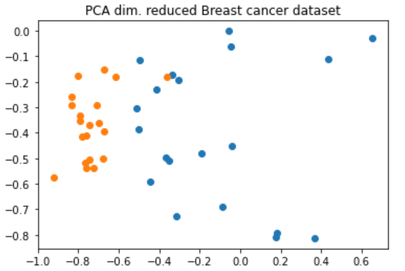
Now, the PCA dimension reduced breast cancer dataset is shown in Figure 15. It can be seen that there are some overlap in the data. These were the training dataset. The classical and quantum machine learning algorithm is needed to be trained first to analyze the performance of VQC.
Breast cancer dataset is reduced in dimension to two for computational advantages. PCA algorithm has been used to take the best two features of the data to solve this classification problem. At first, the classical ML algorithm has been applied to this problem and the result is checked with IBM lab document. In IBM lab document, they have used a different approach to analyze and solve this classification problem. The first part of the table 4 below shows that
| SVM | QSVM | |
|---|---|---|
| Breast Cancer Analysis | 85% | 90% |
Table 5: Performance analysis of Classical and Quantum ML algorithm on other dataset with IBM Lab document [9].
classical SVM has got 85% accuracy and with QSVM, IBM has got 90% of accuracy. So, quantum enhanced support vector machine performed better than classical algorithm for this case. However, the improved version of the optimized VQC algorithm is needed to be tried on this dataset. All the optimizers have been tried to test and to understand what optimizer works better. In the findings, it has been found that COBYLA and TNC perform better than the classical SVM algorithm. Table 4 illustrates the performance of classical and quantum machine learning algorithm.
| Optimized VQC | ADAM | AQGD | COBYLA | SLSQP | TNC |
|---|---|---|---|---|---|
| Breast Cancer Analysis | 50% | 85% | 90% | 50% | 90% |
Table 6: Performance analysis of Classical and Quantum ML algorithm on other dataset with IBM Lab document [9].
The performance of optimized VQC on PCA dimension reduced breast cancer test dataset can be illustrated in the Figure 16.
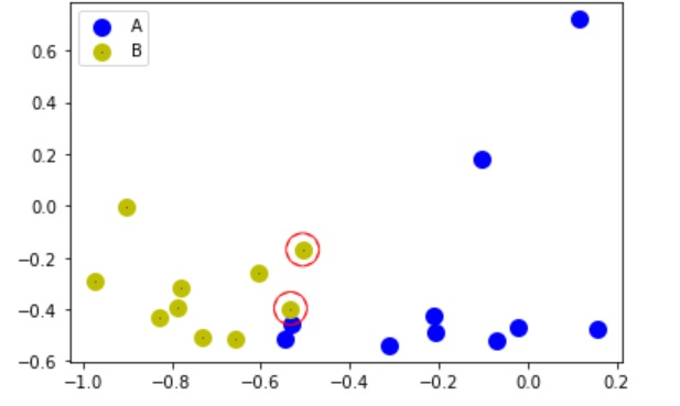
From Figure 16, it can be found that there are only two data points that are misclassified. Others are classified properly. From table 4, it can also conclude that SLSQP does not always perform well as claimed earlier. COBYLA also has performance issue in some settings as shown in figure 12. But TNC optimizer always performs better than all the other classifier. So, the TNC optimizer is recommended to build this optimized algorithm.
Optimized Algorithm
The optimized VQC classifier is as following:
- Data set loading
- Distributing train and test dataset xi by Class
- Initiating statevectors as per feature space=n
4. Initializing Z Feature map with depth 2 5. Initializing RealAmplitude with depth 2 6. Combining Z Feature map with RealAmplitude 7. Function for data dictionary Pass in: parameter, data Initiating blank parameter dictionary For i, p ϵ ordering parameters for Z Feature map do Assigning parameters for each data point End for For i, p ϵ ordering parameters for RealAmplitude do Assigning parameters for each RealAmplitude rotation gate End for Return parameter dictionary 8. Function assign label Pass in: bit string, class labels For k ϵ bit string list do hamming weight= sum of all bit string End for Defining odd parity IF Odd parity THEN Return assign label 1 ELSE Return assign label 0 9. Function return probabilities Pass in: counts, class labels Initiating dictionary for Assigning labels For key, item ϵ items count do Calling assign label function Pass in: key, class labels Calculating total probability of getting one label End For Return total calculated probability 10. Function Classify Pass in: data, parameters, class labels Initializing state vector empty list For x ϵ data do Assigning data and parameters by function data dictionary Updating state vectors Adding updated state vector to empty list End For Initializing empty class probability list For qc ϵ state vector list do Counting return measurement probability dictionary of quantum circuit Calling return probabilities function Pass in: Counts, class labels Adding class probability list Return class probability list 11. Function Sigmoid Pass in: probability list, expected labels Calculating probability of expected label IF probability of expected label is close to 1 THEN Assign 0 ELSE IF probability of expected label is close to 0 THEN Assign 1 ELSE Calculate and assign 1 / (1 + math.exp(-x)) Return Assign 12. Function Cost function Pass In: training input, class labels, parameters, shots number Initiating training labels empty list Initiating training samples empty list For label, samples ϵ training input items do For samples ϵ samples do Adding training label to empty training labels Adding training samples to empty training samples End For End For Calling classify function for the value of probability Pass In: training sample, parameters, class labels For i, probability value ϵ enumerate probability values Calling sigmoid function for calculating Cost Pass in: Probability, training labels index value End For Determine overall average Cost Return overall average Cost 13. Assigning TNC optimizer with maximum iteration= 100 14. Creating objective function by calling cost function Pass In: training input, class labels, parameters 15. Initiating random parameters 16. Optimizing parameters by calling optimizer function Pass In: length of initial parameters, objective function, initial parameters
Conclusion
From this study, it can be concluded that an optimized VQC can be developed to solve classification problem by analyzing the behavior of its components. Z feature map should be chosen as the encoder with circuit depth 2.
The ansatz of this study can be used as the tuning circuit which must also have depth 2. Additionally, TNC optimizer will help to obtain the best possible results from the VQC. This optimized VQC performs similar or better for lower dimensional dataset provided that the physical quantum computer is ideal or qubits are totally immunized from noise.
References
-
Schuld M, Sinayskiy I, Petruccione F (2015) An introduction to quantum machine learning. Contemporary Physics 56(2): 172-185.
-
Wittek P (2019) Quantum Machine Learning MOOC. University of Toronto, Spring.
-
Wittek P (2014) Quantum Machine Learning What Quantum Computing Means to Data Mining. 1st(Edn.), Elsevier, pp: 1-176.
-
Havlicek V, Corcoles AD, Temme K, Harrow AW, Kandala A, et al. (2019) Supervised learning with quantum enhanced feature spaces. Nature 567: 209-212.
-
Preskill J (2018) Quantum Computing in the NISQ era and beyond. Quantum 2: 79.
-
Hubregtsen T, David W, Elies GF, Peter Jan HSD, Paul KF, et el. (2021) Training Quantum Embedding Kernels on Near-Term Quantum Computers. Quantum Physics 1: 1-19.
-
Schuld M (2021) Supervised quantum machine learning models are kernel methods. Quantum Physics 1: 1-21.
-
Abbas A (2020) Basic programming for quantum machine learning with Qiskit and PennyLane. NIThep Mini School, University of Kwazulu-Natal, South Africa.
-
Asfaw A (2020) Learn Quantum Computation Using Qiskit.
-
Stein SA, Mao Y, Betis B, Daniel C, Ying M et al. (2021) QuClassi: A Hybrid Deep Neural Network Architecture based on Quantum State Fidelity. Quantum Physics 1.
-
International Business Machines Corporation (IBM) (2022) Torch Connector and Hybrid QNNs.
-
(2022) MNIST Classification.
-
Macaluso A, Luca C, Stefano L, Claudio S (2022) Quantum Ensemble for Classification. Computer Science > Machine Learning 1: 1-19.
-
Kothari V (2021) QML for image processing. QIntern, Project 19.
-
Wang Z, Zhiding L, Shanglin Z, Caiwen D, Yiyu S, et el. (2021) Exploration of Quantum Neural Architecture by Mixing Quantum Neuron Designs. Quantum Physics 7.
-
Winston P (2010) Learning: Support Vector Machines. MIT Artificial Intelligence.
-
Priyadarshiny U, DZone (2019) Introduction to Classification Algorithms. Dzone.
-
Qiskit Development Team (2020) IBM, Qiskit Challenge India.
-
Qiskit Development Team (2021) IBM, Class Lecture, Quantum Computing, Quantum Machine Learning. Qiskit Global Summer School on Quantum Machine Learning.
-
Qiskit Development Team (2020) IBM, Qiskit Challenge India.
-
Zheng M, Holton S, Ouyang J (2020) Quantum Support Vector Machine.
-
Nielsen MA, Chuang IL (2010) Quantum Computation and Quantum Information. 10th Anniversary (Edn.), Cambridge University, pp: 1-704.
-
Wu Y, Juan Y, Pengfei Z, Hui Z (2021) Expressivity of Quantum Neural Networks. Condensed Matter > Disordered Systems and Neural Networks.
-
Sim S, Johnson PD, Aspuru Guzik A (2019) Expressibility and entangling capability of parameterized quantum circuits for hybrid quantum-classical algorithms. Advanced Quantum Technologies 2(12): 1900070.
-
Qiskit Development Team (2021) IBM, Qiskit 0.36.0 documentation.
-
Ravi J (2018) Machine learning-Iris classification.
- Lessons to Learn: Trees are More than the Lungs of the World
- Community Forestry Enterprises as a Model for Sustainable Forest Development: The Case Of The "Baja Tarahumara" in Chihuahua, Mexico
- Ecological and Socio-Economic Impacts of Chromolaena odorata and Mesosphaerum suaveolens, Two Invasive Alien Species in Central and Southern Benin, West Africa
- Epigenetic Sustainability: Modeling the Human Factor as a Natural Resource through Science 4.0 and the NR3C1 Biological Pilot
- Growth-at-Risk: A Framework for Assessing Economic Vulnerability
- The Rural Territory as a Socioecological System for the Management of Public Policy for Sustainable Rural Development