Development of the Covid-19 Epidemic Model: Calculations for a Mutating Virus

Introduction

A large number of studies have been devoted to the development of models describing epidemic growth. With the development of computer technology and programming methods, these models have been steadily increasing in complexity. However, their operational use in practice has not found wide application due to the need to use rather cumbersome numerical methods, but, more importantly, these models require for their realization the introduction of a large number of experimental coefficients. Under these circumstances, it would be desirable to develop a simple model that would adequately describe the patterns of epidemics. With the help of such a model, it would be possible at the administrative level to make operational decisions both to prevent epidemics and to develop an optimal strategy to reduce them.

The model we propose has shown good efficacy in the initial stages of the COPD 19 epidemic [1, 2, 3, 4]. However, as the epidemic evolves, there is a need for further testing and development of this model. The present work is devoted to developing the model and refining it at a later stage of epidemic growth.

Methodology

The initial equations that were used to derive the computational dependencies are of the form [1]:

0 dl S I k dt N × = × (1)

ds S dt λ = −× (2)

In which: I - number of infected persons at a given time, 𝑘0 - Corona virus infection rate (1/day), N - Total population of the area under consideration, S - Number of susceptible part of the population potentially capable of becoming infected due to contact with infected individuals.

In the models usually used to calculate the growth of the epidemic [5] it is assumed that the value of S is constantly decreasing due to the growth in the number of infected persons I and therefore the system of equations can only be solved by numerical methods. In the proposed simplified model, it is assumed that, provided that S ≫ I, the growth of infected patients has almost no effect on the value of S. The number of persons capable of contracting the virus depends only on quarantine conditions:

0 t S S e λ − = × (3)

In which: 𝑆0 is the maximum number of potentially infectious persons and λ is the intensity factor of decrease in contacts of infected patients with persons who potentially can get infected by means of quarantine and other preventive measures.

As has already been established in our previous works [2, 3], the transition from the absolute number of infected to their relative number per inhabitant allows us to obtain universal dependences that agree well with the statistical data for both small regions and large countries. Let us write down this basic calculated dependence in the form:

( ) 0 100 *exp 1 rk t i i e N λ λ   − = + −    

(4) In which: 𝑖 - Relative number of infected persons per one inhabitant of the settlement in question, as a percentage, 𝑖0 - Value of 𝑖 at the initial moment of the calculation period, k - Transmission rate coefficient for the settlement with a population of N, which is calculated by the formula:

6 1 0,355 0,035*ln *10 K N   −   =  

(5) This formula was obtained for the virus strains responsible for the so-called first and second waves of the epidemic. As for the third wave, actively spreading in the United Kingdom and several other countries since January 2021, it is recommended to increase the first summand in (5) to 0.38 1/day due to more active transmission of the new strain [6].

The other coefficient used in the proposed model, λ, is determined by the rigidity conditions of the quarantine. As control calculations have shown for a number of cities and countries in Europe, as well as the USA, it turns out to be quite stable and equal to λ = 0.035 1/day [3, 4]. At the same time, a situation often arises when, as a result of insufficient measures to reduce the growth of the epidemic, the spread of infection gets out of control. In this case, there is a need for a drastic change in quarantine. Conditions such a situation occurred, for example, during the first wave of epidemics in Spain, Italy and in some cities in the United States, particularly in New York. When using the proposed model, a new value of the coefficient λ must be introduced into the calculations, starting from the time when stricter quarantine measures are adopted.

Let for the time period 0≤ t ≤ t1 assume that λ = λ1, and for t >t1 this coefficient changes to λ = λ2. Then the calculation is first performed by the basic relation (4) including until the time t1. The further calculation is carried out by the relation, which takes a slightly different form:

− −   = + + −    

( ) ( ) 2 1 2 0 1 0 2 *exp t t k i i i i e e λ λ λ (6)

𝑖1 and 𝑖0 are the relative numbers of infections at time t = t1 and at t = 0, calculated by (4) with the coefficient λ = λ1. This relationship can be useful in analyzing the rate of epidemic growth during and after major holidays, e.g., Christmas, Easter, etc. Ratio (6) is obtained by integrating equations (1) and (2) under the following conditions: t = t1, i = i1.

Relatively intensive changes in the rate of spread of the epidemic can be related not only to changes in quarantine conditions, but also to the possibility of new strains of the virus. In this situation we can assume that the growth of the infection depends on the spread of both types of virus simultaneously. Then the calculations can be performed according to the following dependence [3].

( ) ( )           = + +                

0 100 * exp * 1 e * xp 1 n n k k i t t t e e i N λ λ λ σ λ − − − − −      

(7) 𝑘𝑛-Transmission rate coefficient of the new virus strain and the time of the epidemic wave associated with the new coronavirus strain σ tn - start time of the new epidemic wave associated with the new coronavirus strain σ - Heaviside symbol: σ = 1 when t ≥ 𝑡 1 and σ = 0 when t < 𝑡1.

Ratio (7) is obtained under the assumption that the two virus species exist independently of each other. This assumption may not hold for certain strains of the virus, in which case the calculation is performed as a sequential replacement of one virus species by another. If there is a sharp increase in the rate of spread of the virus, it can sometimes be quite difficult to establish the true cause of such changes, i.e. to determine which of the two dependencies should be used to calculate the growth of the epidemic.

Results

An analysis of the spread of the epidemic in several countries of Europe and the United States shows [3], that since mid-December 2020 there has been a significant increase in the rate of infection, which may be related to the relaxation of the quarantine conditions at Christmas and to the appearance of a new virus strain which was detected at least in the United Kingdom in October 2020 [7]. Let us try to find out the cause of these changes using relations (6) and (7), using the United Kingdom and South Africa as an example. The differences in the character of the changes in the intensity of the epidemic growth are related to the fact that in case a new strain of the virus appears, we can expect its longer impact on the spread of infection than in case of a relatively short-term decrease in quarantine conditions during the holiday period. Benchmark calculations using both methods for the United Kingdom were made.

Click to enlarge

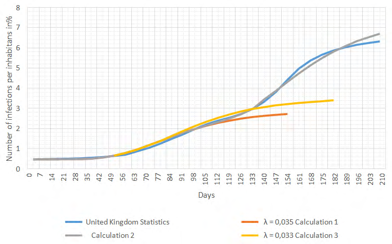
Figure 1 represents statistical data [8] for the epidemic development from the beginning of so called second wave, which is from August 08, 2020 to March 12, 2021 (time of writing this work). The same figure shows the results of calculations. Calculation 1 was performed according to the dependencies (4) and (5) for the coefficient λ = 0.035 1/day.

As we can see from the comparison of the calculation results with statistical data, the calculation quite well describes the development of the epidemic up to a certain point in time (up to the middle of November 2020). But already at the end of November, i.e., about 100 days after the beginning of this epidemic wave, there is a noticeable divergence in the data. Calculation 2 was performed using dependences (4) and (6) at values λ1 = 0,035 1/day and λ2 = 0.033 1/day. In these calculations the assumption was made that quarantine restrictions were relaxed in mid-December due to the coming of Christmas, which led to an increase in the epidemic in the United Kingdom. The calculation under this assumption showed some increase in the number of infected patients, but the results of this calculation also do not agree well with the statistics. The introduction of other, lower values of the coefficient λ into the calculations does not fundamentally change the situation. The growth patterns of the epidemic in the United Kingdom cannot be described by using ratios that assume that only changes in quarantine conditions are taken into account.

If one assumes that a new virus species significantly different from the “old” strain is emerging along with it, then the calculation must be carried out according to relation (7). The results of such a calculation (calculation 2) are presented in Figure 1. Quite good not only qualitative but also quantitative correspondence of the data confirms the validity of the assumption about the appearance of a new virus variant at time t1 (beginning of December). The calculations were performed with the previously accepted coefficient λ = 0.035 1/day, i.e., quarantine conditions were assumed unchanged for the entire epidemic growth period.

The coefficient characterizing the transmission rate of the virus was calculated according to ratio (5) and was equal to K = 0.5 1/day. Considering, however, that a study of this new virus species [6] (strain B 1.17) revealed its transmissibility to be markedly higher than that of the former species, this coefficient was increased to K = 0.52 1/ day. The United Kingdom was chosen as an example because of the large number of studies on the characteristics of the epidemics associated with this new strain, sometimes called the “English virus” [6] in various countries. In addition to this type of coronavirus, the “South African” and “Brazilian” varieties of the virus are also widespread in several countries.

Click to enlarge

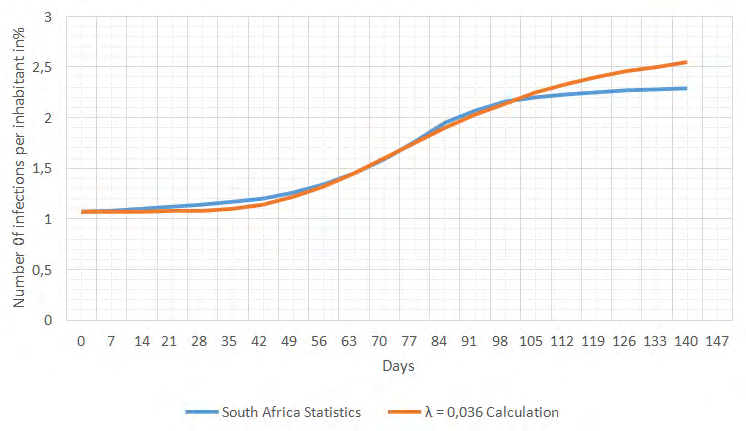
As a second example of applying the model, the spread of the epidemic in South Africa was calculated. Initial statistical information on the growth of the epidemic in South Africa is given in [8]. Figure 2 shows the epidemic spread of COVID 19 from October 23, 2020 to March 12, 2021.

Comparison of estimated and statistical data shows their good correspondence for the period from the beginning of the epidemic wave in question to the end of January 2020. It should be particularly noted that during the whole period in question the epidemic development rate is somewhat lower than that for countries and cities in Europe and America. The coefficient λ characterizing the effectiveness of quarantine for South Africa turned out to be higher (λ = 0.036 1/day) i.e. the transmissibility is correspondingly lower than for most cities and countries. Starting from the middle of February, the divergence of the data is observed, and the epidemic develops significantly weaker than it is determined by the calculation. It is possible that this difference in the rate of spread of the epidemic in South Africa can be explained by the peculiarities of the genome of this strain of the virus. A detailed study of the changes in the properties of the virus strains during the whole epidemic shows in particular that during the month from October 5 to November 2, 2020, the virus strain known as “South African” B1.1.351 (501YV2) has completely superseded all the other strains of the virus [9]. Interestingly, the rate of these changes was so high that it was not necessary to use a two-strain model to calculate the spread of the epidemic. At the same time, it can be deduced from comparing these results that the virus strain dominating in South Africa was significantly less transmissible than, for example, the “English” virus B1.1.7. The decrease in the growth rate of the epidemic since February 2021 cannot be explained by the influence of vaccination, since the vaccination rate in South Africa did not exceed 0.5% in mid- March. The reasons for these differences will have to be further established.

Click to enlarge

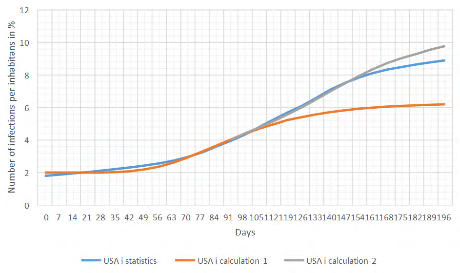
Figure 3: Prevalence of the epidemic in the United States. One country in which there has been a particularly active spread of the virus is the United States of America. Figure 3 shows comparison of statistical and calculated data for the USA. In general, the calculated and statistical data agree with each other quite satisfactorily. The epidemic is characterized by a high growth rate; therefore, a relatively low value of the quarantine efficiency coefficient λ = 0.034 was assumed in the calculations. The K coefficient, which takes into account virus transmissibility, was assumed to be the same for each epidemic wave in accordance with the results of calculations using formula (5).

Discussion

Overall, the proposed computational methodology quite adequately describes the patterns of virus spread under different conditions. It is not entirely clear how one could explain why, starting from February 2021, the epidemics in the countries in question are spreading with much less intensity than the model predicts. For the United Kingdom and the United States, there is no doubt that the course of the epidemic is strongly influenced by the mass vaccination of the population, but this factor should have no influence on the development of the epidemic in South Africa. Apparently, there is an influence of an as yet unknown factor. It could be assumed that the proposed model does not take into account that as the proportion of the population that is infected increases, the number of people potentially exposed to the virus decreases. However, we have to keep in mind that for South Africa, the total number of infected people over the entire period of the epidemic, does not exceed 2.5%. It is difficult to assume that such a low percentage of infected people can affect the number of potentially infectious individuals. In order to reasonably establish the factor responsible for the decline of the epidemic, starting in February 2021, it is necessary first of all to trace the further development of the epidemic. And of course it is necessary to introduce adjustments into the model, taking into account the rate of vaccination of the population. Mass vaccination should undoubtedly slow down at some stage, and then stop the epidemic completely.

As indicated earlier, two empirical coefficients are used in the model. One of them, the coefficient determining the transmission rate for most coronavirus strains, can be calculated according to formula (5) and depends mainly on population size. Only for the last wave of epidemics in the United Kingdom was this coefficient slightly increased compared to its value for the previous wave. It might also be possible to increase this coefficient when calculating the growth of an epidemic in the United States. However, this question should be considered in relation to the intensity of transmission of the main virus strain. Such studies are based on the genome sequencing of the virus and are carried out in many research centres. A generalization of the results of these studies will allow, among other things, a more reliable determination of this coefficient for each strain.

A more difficult task is to choose the coefficient λ, which depends on the effectiveness of measures to reduce the rate of transmission, which for simplicity we will call the effectiveness of quarantine E. These measures include: compulsory wearing of masks, compliance with distancing, reduction of contacts, and hand hygiene. A large number of studies have been devoted to analysing the impact of each of these factors. In particular gives an overview of studies on the effectiveness of the different masks, on the effectiveness of keeping a distance. Each of these factors depends to a large extent on age [10]. For example, the amount of contact for school-age children is largely determined by school conditions. Similar conclusions for each age group, denoted by the index “n,” would allow a more reliable analysis of the effect of each of the main factors for each age group on the intensity of the epidemic. As a very rough estimate, the quarantine effectiveness coefficient can be estimated using a simple formula:

n n n Q C p e p d p h µ − − − = ∑ (8)

m

1 2 3 * * 1 * * 1 * { ( ) ( ) * 1 } * ) ( n n In which: pn1, pn2, pn3 – parts of the population in each age group n that comply with the rules of mask wearing, distance keeping (at least 1 m) and hand hygiene, e, d, h, Cn – effectiveness of masking, distance, hand hygiene, and reduction in contact, m – Total number of age groups, μ - proportion of the population of a given age group relative to the total population, i.e. 𝑁𝑛 𝑁 From ratio (4) determine the maximum total number of people who were ill with the virus during the epidemic:

0 100 *exp rk i i N λ   = +    

(9) Since relation (4) and respectively (9) is universal and the relative number of infected does not depend on the number of inhabitants (3), but is determined only by the value of λ, we can obtain a relationship for the relationship of this coefficient with the lockdown efficiency coefficient. Fig. 4 shows the graph of the dependence of λ on the parameter E = 1 – Q (Figure 4).

Click to enlarge

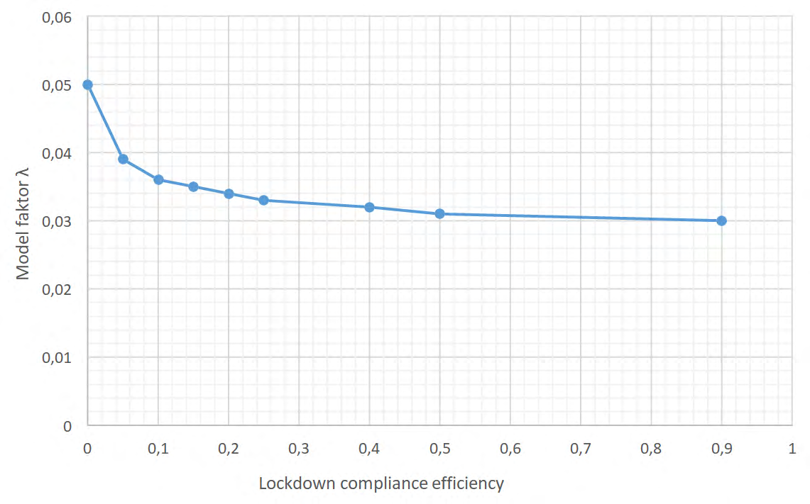
From the graph, in particular, we can determine that the value of coefficient λ = 0.035 1/day approximately corresponds to the value E = 0.2 or Q = 0.8.

The justified choice of model coefficients depending on the number of inhabitants, virus transmissibility and lockdown conditions makes it possible to use the proposed model not only as a calculation model but also as a forecast one. Thus, it is possible to predict the growth of the epidemic depending on the main factors. However, it should be borne in mind that these dependencies may differ significantly for different countries, depending on the ethnic composition of the population, traditions and the psychological perception of lockdown requirements.

Conclusion

• A method for calculating epidemic growth under conditions of simultaneous action of several virus strains is proposed. Comparison of calculation results on proposed ratios for countries with intensive recurrent epidemic growth due to virus mutation is in satisfactory agreement with statistical data.
• The method of calculation of epidemic growth under sharp changes of lockdown conditions is developed. To confirm the possibility of using this method it is necessary to compare the results of calculations with the data of statistics.
• When the results of the calculations are compared with statistical data, a systematic bias is observed from late February and early March onwards. For countries where vaccination is intensively carried out, this deviation can be explained by a decrease in the proportion of the population that can be infected by contact with infected persons. However, such differences for South Africa, where intensive vaccination is not carried out, require further investigation.
• In order to develop the model further so that it can be used not only for calculation but also for predicting the spread of the epidemic according to the main factors, a link is established between the coefficient of the model and a parameter characterizing the level of lockdown, i.e. the quarantine-efficiency coefficient. In the future, this coefficient will be related to the level of compliance with quarantine rules.