Stability in Food Security within the Southern African Customs Union: A Dynamic Panel Analysis Approach pn Cereals
Food insecurity is no different in southern Africa. This paper attempts to assess the country effects within the aggregated cereal food security status within the Southern African Customs Union (SACU). The impact of a big player on dependent small players is analysed by using the panel data approach to empirically explain the dynamics of climate patterns on cereal food production. The paper employed econometric dynamic models to determine effects of urbansisation, production yield, land availability and weather variables on both country individual and regional food security. Results indicates that a unit decrease in available crop surface per capita in each time period leads to 40% decrease in the ability to be food secure within the SACU region. It implies that countries with less crop surface, low crop yield and high population growth tend to be less food secure because of applying less rigorous food production technologies. Therefore, adjustments in cereal food production in Southern Africa are necessary to follow principles of climate smart agriculture. Resulting shifts in production systems will open an opportunity for regional cooperation in food resource management. Iindividual country policy on food security shows divergence and could be adjusted towards a more holistic regional approach with innovation, trade, health, wealth and geopolitical relations. Individual country support from a regional customs union will strengthen regional equity and sustainable development for ultimate welfare. Technological change in cereal food production practices will be based on resource quality and management skills.
Introduction
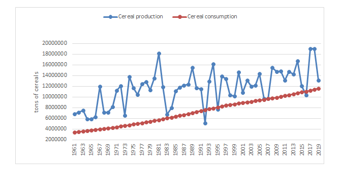
The concept of increasing food insecurity is well established [1, 2, 3]. Almost 15% of the global population does not have enough to eat, while global food production continuous to kept ahead of demand [4]. The deficiencies of food availability, accessibility, utilization and stability have to be addressed to advance human wellbeing and development [1], by applying rigorous systematic analysis. Literature show many causes of insecurity, such as effects of urbanization, globalization, trade regulations, consumption patterns, diseases, adverse climate conditions on food production, land degradation, water scarcity [2, 5, 6], which additionally might have caused some volatility in global food prices of underdeveloped countries. The factors leading to shortages in food supply and consequently on the food security will be investigated to determine impacts on regional food security in Southern Africa. Similar than the aggregated global situation, Southern Africa produces more than consumed, but disaggregation shows insufficiencies. Figure 1 presents the narrowing case of cereal security and how its volatility affects food security.
Resent COVID-19 restrictions exposed the definition on food security1, namely that intraregional trade restricted food security in Southern Africa. Frictions within this definition have to be understood to allow proper quantity and quality security Adams RM, et al. [7], especially when aggregated under the Southern African Customs Union (SACU). As the developmental status of its member countries are very diverse, with only South Africa being a net cereal exporter, special attention is required to allow equity within food security. Table 1 demonstrates the dominance from South Africa in terms of commodity exports and comparative advantage2,
1 Food security exists when all people, at all times, have physical and economic access to sufficient, safe, and nutritious foods that meets their dietary needs and food preferences for an active and healthy life (Food Summit, 1996).
2 The RCA for vegetable products (AATM, 2020) was used to show the food security aspects within SACU. Countries with relative disadvantages, such as Eswatini, and Namibia decreased their RCA continuously from while cereal dependency is observed in Botswana, Eswatini, Lesotho and Namibia. The relative comparative advantage (RCA) for vegetable products was used to show food security rankings within SACU. Countries with relative disadvantages, such as Eswatini and Namibia showed worsening of low RCA from 2003-2018, while Botswana and Lesotho presented a high volatility within their disadvantages over time [8]. Within SACU, South Africa was the only country with relative comparative advantage, although it showed to be volatile over the period. Furthermore, Table 1 also compares the urbanization of the member countries; high in Botswana, Namibia and South Africa, while low in Eswatini and Lesotho with their smaller economies.
2003 to 2018, while Botswana and Lesotho presented a high volatility over that period. Within SACU, South Africa is the only member with vegetable products relative comparative advantage, which is also showed to be volatile over the period.
| SACU member country | Intra-regional trade imports 2018 (R bill) | Intra-regional trade exports 2018 (R bill) | Revenue share (2018) | Urbanisation (2019)* | Average relative comparative export advantage on vegetable products (2018)** |
|---|---|---|---|---|---|
| Botswana | 68.7 | 9.6 | 21.30% | 70.17% | 0.06 |
| Eswatini | 16.9 | 16.9 | 6.40% | 23.80% | 0.39 |
| Lesotho | 16.2 | 4 | 6.10% | 28.59% | 0.37 |
| Namibia | 61.1 | 23.4 | 19.10% | 51.04% | 0.42 |
| South Africa | 37.8 | 146.7 | 47.10% | 66.86% | 1.64 |
| Total | 200.6 | 200.6 | 100% |
Table 1: Summarised comparison of SACU member countries. Source: Adapted from SACU (2019) and AATM (2020)** [8].
This paper attempts to analyze food security by using a regional case and to determine the impact of a big player on dependent small players. The panel data approach is used to empirically explain the variables dynamics on cereal food production resulting into food security. Results are used to support climate smart technical processes and to become more resilient [9, 10]. An attempt is made to direct food security between SACU and the individual countries’ stability.
Empirical Background
Food security is not only a systemic challenge in Southern Africa, but maybe an opportunity for SACU to play a role in innovation, trade, health, wealth and geopolitical relations. SACU, formed in 1910 for trade integration, primarily focus is on trade facilitation and revenue management, with a defined vision of equitable and sustainable development. This unintentionally allows them to contribute towards improved food security for member states and calls for policy coherence and the development of common strategies towards welfare of its citizens. Therefore, the trade occurrence, depending on proximity, cultural similarities, and trading relationships [11], might be adjusted to reduce the food insecurity.
Conventional wisdom states that food security becomes a concern only once the population growth exceeds the growth in production. However, as the resources are limited, and urbansisation and climate changed entered the equation [12], the consuming society will increasingly depend on technological change to overcome this problem. For the SACU countries three countries are selected, namely South Africa, Botswana and Namibia. Their cropland per capita did not only decline over time, but environmentally differs as such that the setting in South Africa on average has three times more cropland available per capita than Namibia and Botswana.
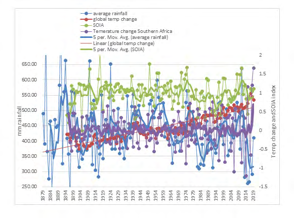
Akpalu W, et al. [13] showed that the amount of precipitation is the most important crop production driver in South Africa. For maize, they found that a 10percent reduction in mean precipitation reduces the mean maize yield by approximately 4percent. They determined that the mean temperature increase from 21.4-21.6 degrees Celsius, which resulted into average yield increases by 0.4percent. This is different to the time series data used in this paper from 1879-2019 (Figure 2), showing that precipitation declined with 0.32mm annually, while mean temperature increased with 0.13degree Celsius annually. Using these long-term general trends, it is important to understand that crop yields may diminish based on the weather effects, especially as the magnitude and the direction of climatological variables change. In this regard, Conradie B, et al. [9] found that temperature is becoming a lead production determinant, and suggest that the disaggregation and availing of weather data is necessary in the discussion on food security.
Figure 2 shows that the global temperature change is significantly more than those observed for Southern Africa. It is observed that the amplitude size for average temperature is increasing over time. The weather variables Southern Oscillation Index Average (SOIA) and average rainfall in Southern Africa show a cyclical movement over the past millennia. Individual weather stations showed an increased combined score of the rainfalls’ coefficient of variation, which increase over time implies that the volatility gets worse with highest volatility since 2000. All these trends clearly have to be known to determine the impact on food security.
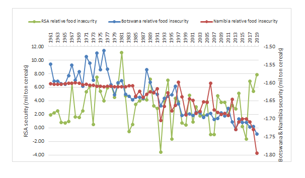
Secondary country data of cereal production for Botswana, Namibia and South Africa, were used to illustrate the relative effect by countries. Figure 3 shows changing cereal food security over time. It shows that Botswana and Namibia are net importers of cereals, resulting into negative security, while South Africa is mostly a net exporter of cereals, resulting into positive security. The change of security over time was analysed by applying the t-test on paired sample means to determine the significance of change over time. For South Africa, it is evident that the fluctuating mean cereal food security declined with 33% (t=1.81) between the period 1961-1990 and the period following 1990, while Botswana became 6% more secure (t=11.89) in the period after 1990, and Namibia more secure with 4% (t=9.57). It is interesting to note that in relative terms, the SACU’s main cereal supplier shows the highest level of increasingly becoming more insecure, while the insecure countries show signs of improvement. Furthermore, the volatility of annual food security has to assess too. The South African coefficient of variance (CV) over time increased with 56%, while the Botswana CV decreased with 22% and Namibia show an increased CV of 260% since 1990.
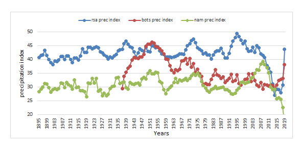
Some of the increasing changes in (in) security is believed to be the result of weather effects resulting into changing cereal production, which cyclical pattern is hinted in Figure 4. Changes might have resulted into the shifts of production systems, such as from crops to livestock [14], affecting farm incomes Kurukulasuriya P, et al. [15], with implied famine and health concerns López-Carr D, et al. [16]; Speranza CI, et al. [17].
Kotir JH, et al. [18] shows that Southern Africa show a high dependence on agricultural production as livelihood, which calls for measures complying with the increased climate volatility. Suggested climate smart agriculture focus on disaster risk reduction processes. Reducing risk in food production would generally look into the use of improved crop varieties or agronomic measures [19, 20]. These depend on the understanding of weather variables’ interdependencies to be a useful addition alongside the food security risk reduction measures [21].
The paper suggests incorporating these relative changes to cereal production and becoming climate smart, by understanding the climate variables leading to sustained food security. A series of studies showed positive returns benefiting from climate forecasts in managing the gross margins of in crop production [22, 23]. However, this is only one way to counter the production volatility through applied climate information systems [24]. For individual countries within SACU, it is essential to address the annual volatility in cereal trade needs to improve food security. The next section will present the methodology by pooling effects to estimate the relationship among these variables, required to determine the impact such as global climate change on food security in the Southern Africa.
Methodology
In principle it should be simple to determine which variables explain the changing levels of food security. However, some variables are secondary such as climate change [25] impacting on food production. The complex interplay among weather variables is not always straightforward. Baten A, et al. [26]; Solís D, et al. [27] for example proved that precipitation is not necessarily statistically significant with the expected sign, nor does it show the direction of causality [28]. Thus, the thrust of this study was to assess the impact of multivariate factors on regional food security in selected SACU countries. In order to achieve this objective, an econometric analytical technique was applied on panel data based on the three countries covering the period from 1961-2019. This method allowed for the joint analysis of the cross-sectional data over the time period producing rich and more robust results to conclude on the impact of regional integration on food security and socio-economic development in the SACU region. This section begins with explaining the s nature of data used. In addition, the next section describes the data analysis starting with the panel unit root tests for data stationary. Then a more in-depth review of the Least Square Dummy Variable (LSDV) technique, the fixed and random effects models applied in this study.
Data Characteristics
This study employs panel data from Botswana, Namibia, and South Africa, covering the sample period from the year 1961 to 2019, and therefore generating a balanced stacked panel of 177 observations (time period = 59 and across 3 countries). The choice of the period under study was mainly influenced by the fact that following the notable developments of attainment of Namibia’s independence in 1990 and the ending of apartheid in SA in 1994, SACU member countries entered into new negotiations leading to the new SACU agreement of 2002. This agreement addressed issues of enhancing equal participation by members, the new revenue sharing formula and the need to develop strategies that would strengthen their integration without jeopardizing the economies of the smaller economies and ensure food security. This paper uses climate data to determine impacts on regional food security in Southern Africa to suggest policy adjustments.
Data were obtained from the SACU statistical database, the World Bank database of production and cereal consumption are obtained from national statistical offices, implying desktop data extraction as a data collection method. Table 2 provides a brief overview of data sources employed.
| Variable | Code | Definition | Source |
|---|---|---|---|
| Cereal consumption | CERCONS | Total population multiplied by individual annual cereal consumption | https://data.worldbank.org/indicator/SP.POP.TOTL?locations; and https://www.helgilibrary.com/indicators/cereal- consumption-per-capita-excluding-beer |
| Cereal Production | CERPROD | Total annual cereal production in tonnes | https://knoema.com/atlas/country/Cereal-production, and https://www.researchgate.net/publication/338212708 |
- Population
- LPOP
- Natural logarithm of the total population https://data.worldbank.org/indicator/SP.POP.TOTL?location
- Trade index
- LTI
- Natural logarithm of relative cereal volume traded among
- SACU member countries
- Obtained from above sources surface per capita
- SHC
- Cereal crop surface divided by the country population http://www.fao.org/faostat/en/#data/QC
- Indication of the development and intensity of El Niño or La Niña events in the Pacific Ocean
- Southern
- Oscillation
- Index Average
- SOIA
- Rainfall
- LRAIN
- Natural logarithm of annual rainfall in mm
- Temperature
- LTEMP
- Natural logarithm of average monthly temperature aggregated to annual
- Yield per hectare
- YHA
- Total cereal production divided by cultivated cropland for cereals.
- Obtained from above sources
- Yield per rural population
- YRPOP
- Cereal production divided by (total population minus urban population)
- Obtained from above sources
- Urban population
- URBPOP
- Total country population multiplied by urbanisation rate
- Obtained from above sources
- Effective precipitation
- EFFPRECIP
- Square roof of (average rainfall multiplied by annual average temperature)
- Obtained from above sources
Table 3: Variables descriptions and sources
The Levin, Lin and Chu (LLU) Test
Empirical literature [29, 30], state that panel methods for units and cointegration are based on methods developed for a single time series, on the assumption that T →∞. Their advice is taken into consideration in this study. They advise that if the number of observations is small, being less than ten (N is small, such that N < 10), then seemingly unrelated equation methods can be used, and when N is large, the panel aspect becomes more important.
However, this argument invokes the complications that includes the need to control for cross-section unobserved heterogeneity when N is large, asymptotic theory that can vary with exactly how N and T both to go to infinity and the possibility of cross-section dependence. It is also argued that statistics that exhibit non-normal distributions for a single time series can be averaged over cross section to obtain statistics with a normal distribution. Unit-root tests can have low power. However, panel data may increase the power because of having time series for several cross sections. Cameron AC, et al. [31] suggests that unit-root tests are relevant to consequent considerations of cointegration. For clarity, a dynamic model with cross-section heterogeneity is expressed as follows:
, 1 1 , 1 , ... y ` it i i t i i t i t pi it i it y y y z ρ φ φ γ µ − − − = + ∆ + + ∆ + + (1) Where the lagged changes are introduced so that error term ( ) it µ is identical, independent distributed (i.i.d).
By disaggregation, examples of $Z'{it}$ include: individual effects $[Z'{it} = (1)]$ individual effects and individual time trends $[Z'_{it} = (1t)]$ and $\gamma_i = \gamma$ in the case of homogeneity. Therefore, a unit root test of
$$H_0 : \rho_1 = \ldots \rho_N = 1$$
In this study the postulation approach of Levin, et al. (2002) allows to test the null hypothesis against the alternative of homogeneity, such that $H_0 : \rho_1 = \ldots \rho_N = 1$, that is based on pooled OLS estimation using specific first-step pooled residuals, where in both steps homogeneity $(\rho_i = \rho)$ and $\phi_k = \phi_k$ is imposed.
Contrary to Lewin A, et al. [29]; Im KS, et al. [32] instead test against an alternative of heterogeneity, such that $H_a : \rho_1 < 1, \ldots, \rho_N < 1$ for all fraction $\frac{N}{T}$ of the $\rho_1$ by averaging separate augmented Dickey-Fuller tests for each cross section. In unison, both test statistics are asymptotically normal and both assume $\frac{N}{T} \to 0$ so that the time series dimension dominates the cross-section dimension. The panel-based unit root test proposed in this article allows for individual specific intercepts and time trends. Moreover, the error variance and the pattern of higher-order serial correlation are also permitted to vary freely across individuals. In order to compute the panel test statistics, pool all cross sectional and time series observations to estimate the following equation:
$$\tilde{e}_{it} = \delta \tilde{v}_{it-1} + \tilde{\varepsilon}_{it}$$
Based on a total of observations, where $\tilde{T} = T - \bar{p} - 1$ is the average number of observations per individual in the panel, and $\bar{p} = \frac{1}{N} \sum_{i=1}^{N} p_i$ is the average lag order for the individual ADF regressions. Now the conventional regression t-statistic for $\delta = 0$ is expressed by the following:
$$t_{\delta} = \frac{\hat{\delta}}{STD(\hat{\delta})}$$
Where:
$$\hat{\delta} = \frac{\sum_{i=1}^{N} \sum_{t=2+p_i}^{T} \tilde{v}_{it-1} \tilde{e}_{it}}{\sum_{i=1}^{N} \sum_{t=2+p_i}^{T} \tilde{v}_{it-1}^2 \tilde{e}_{it-1}}$$
And
$$STD(\hat{\delta}) = \hat{\sigma}_{\hat{\delta}} \left[ \sum_{i=1}^{N} \sum_{t=2+p_i}^{T} \tilde{v}_{it-1}^2 \right]^{-1}$$
The Levin-Lin-Chu test for unit root is founded on the null hypothesis that assumes that the panel series contains a unit root and the alternative is that the series is stationary. As explained in the previous paragraph, the Levin-Lin-Chu test assumes a common autoregressive parameter for all panels, so this test does not allow for the possibility that some countries’ trade index contain unit roots while other countries’ real trade index do not [31]. In Stata, each test performed by the command $(x_i \text{ unit root})$, this command also makes explicit the assumed behavior of the number of panels and time periods. The Levin-Lin-Chu test with panel-specific means but no time trend requires that the number of time periods grow more quickly than the number of panels, so the ratio of panels to time periods tends to zero. The test involves fitting an augmented Dickey-Fuller regression for each panel; we requested that the number of lags to include be selected based on the AIC with at most 12 lags. To estimate the long-run variance of the series, $x_i \text{ unit root}$ by default uses the Bartlett kernel using 12 lags as selected by the method proposed by Levin, Lin, and Chu.
This section briefly explains the methodological approaches to panel data analysis. Baltagi BH, et al. [33] define panel data as the procedural approach of forming a pool of observations on a cross section of different economies, households and business entities over a number of periods. In this study, data of the five SACU countries covering the period 1961 to 2019 is pooled together for this analysis to form a data set with ninety (177) observations. The data was analysed through OLS (LSDV), fixed effects and random effects modelling.
**Fixed Effects Modelling**
Proponents of panel data analysis such Baltagi BH, et al. [33]; Greene WH, et al. [34] infer that fixed effects (FE) approach is most applicable in cases where the researcher is concerned with studying the impact of variables that change over time. In fact, it looks into the relationship between the determinant factor and the dependent variable within the analysis. It is assumed that each country may be having some distinct characteristics that may hinder the impact of the determinant factor. For example, policy options pursued by a country may influence business practices of domestic companies and their investment options. In the application of fixed effects, the holding assumption is that each of the countries under study has something that can result in a bias or impact on the determinant or the determined variable, therefore, the biases should be controlled. Baltagi
BH, et al. [33] refers to FE as the whole reasoning behind the correlation assumption between the country's error term and the determinant variables.
The FE approach has an advantage of eliminating the impact of those variables which do not vary with time so that the net effect of the determinant variables on the dependent outcome can be assessed robustly. Another most appealing assumption of the FE model is that those factors which do not vary with time are quite different across the member states and do not correlate with the other countries’ characteristics. Like in majority of econometrics analysis, if the error terms are correlated, similarly, the application of FE provides weaker or no robust inferences, since such inferences would be spurious. Meaning the researcher should opt to use random effects approach to model that relationship. The Hausman test provides the rationale for guidance in determining which approach, either the fixed effects or the random effects is best Greene WH, et al. [34].
It is argued that the fixed-effects model helps to avoid bias in the estimated coefficients emanating from the omitted time invariant variables by controlling for their differences across countries. However, there is a distinguishing shortcoming of the features of fixed-effects models that they are unable to uncover the time invariant causes of the determined outcome variables. Greene WH, et al. [34] commends that technical wise, those characteristics in individual countries which do not vary with time are in perfect collinearity with the country dummies. More so, infers that substantively, fixed-effects models are formulated to figure out the causes of changes within the countries because the time invariant variable is constant throughout the countries and hence it cannot be the source of change. The equation representing the fixed effects model is as represented in equation 7:
$$Y_{it} = \beta_1 X_{it} + \alpha_i + \mu_{it}$$
Where, $\alpha_i(i=1,...n)$ is the unknown intercept for each country (n country specific intercepts), $Y_{it}$ is the dependent variable, where $i$ = country and $t$ = time. $X_{it}$ represents the independent variables, where $i$ = country and $t$ = time, $\beta_i$ is the coefficient for the independent variable, $\mu_{it}$ is the error term. In panel cross sectional data, the beta coefficients are interpreted as: “for a given country, as X varies across time by one unit, Y increases or decreases by $\beta$ units” Baltagi BH, et al. [33]; Greene WH, et al. [34] proposes another formulation of the FE model to capture the binary variables. Meaning the equation for the fixed effect model becomes:
$$Y_{it} = \beta_0 + \beta_1 X_{it} + \dots + \beta_k X_{k,it} + \gamma_2 E_2 + \dots + \gamma_n E_n + \mu_{it}$$
Where, $Y_{it}$ is the dependent variable, where $i$ = entity and $t$ = time, $X_{it}$ represents independent variables, $\beta_k$ is the coefficient for the independent variable, $E_n$ is the entity n. Since they are binary, they assume values of 0 and 1, there are n - 1 entities included in the model, $\gamma_n$ is the coefficient of binary regressors, and $\mu_{it}$ is the error term.
Both equations are similar; the coefficient of the slope on X is equal across the countries. The country specific intercepts in equation 1 and the binary regressors in equation 2 come from the unobserved variable $Z_i$, which varies across the countries but not over time. Adding time effects to country specific effects model results in a time and country fixed effect regression model, which can be represented as follows:
$$Y_{it} = \beta_0 + \beta_1 X_{it} + \dots + \beta_k X_{k,it} + \gamma_2 E_2 + \dots + \gamma_n E_n + \phi_2 T_i + \mu_{it}$$
Where, $Y_{it}, X_{it}, \beta_k, E_n, \gamma_n$ and $\mu_{it}$ are defined as above in equation 1 and 2, respectively. $T_i$ is the time, a binary variable (dummy), meaning there are t - 1 time periods and $\phi_i$ is the coefficient for the binary time regressors.
Baltagi BH, et al. [33]; Greene WH, et al. [34] agreed that controlling for time effects whenever unexpected variation or a special event takes place may affect the model outcome. The fixed effects with dummy variables (LSDV model on fixed effects) gives a perfect means to grasp the fixed effects. Therefore, the addition of dummy variable to each country helps the researcher to estimate with specificity the real effect of the independent variables through the control over the unobserved heterogeneity. Therefore, this each added dummy is absorbing the country specific effects.
Random Effects Model
The foundation of the random effects approach is based on the rationale there is randomness in the variation across the countries and they are not correlated to any of the determinants in the model. The main difference between the random effects and the fixed effects is in the question of whether the unobserved country specific effects contain elements that are correlated with the regressors in the model or not Greene WH, et al. [34]. As stated earlier, the advantage of the RE model lies in its ability to include the time invariant variable in the parameter estimation. Random effect (RE) application is conclusive when a researcher strongly believes the heterogeneity in characteristics across countries have a notable impact on the outcome variable. A sufficient condition to account for is that the random effects model includes those variables which do not change with time such as gender, race etc. While in a fixed effects approach, time invariant variables are absorbed by the intercept. RE assume no correlation between the individual countries’ error term and the exogenous variables thereby allowing those variables which do not change with time an explanatory power on the exogenous variables. In developing a RE model, the key is to correctly specify the country-specific characteristics that maybe or may not be associated with the determinant variables. However, the challenge of correctly specifying the individual characteristics may not be feasible because of unavailability of variables. This then leads to omitted variables’ limitation syndrome and biasness in the model. Baltagi BH, et al. [33]; Greene WH, et al. [34] agree that RE modelling framework enables the generalization of the inference beyond the sample considered in the analysis. The random effects model can be represented as follows:
$$Y_{it} = \beta_{it} X_{it} + \alpha_{it} + u_{it} + \varepsilon_{it} \tag{10}$$
Where: $Y_{it}, \beta_{it}, X_{it}, \alpha_{it}$ and $\mu_{it}$ are defined as before in the fixed effects model. But $\mu_{it}$ accounts for the between countries error and $\varepsilon_{it}$ accounts for the intra country error term. These are included in the empirical equations 1 to 10. The assumption on the errors is that, the country error terms are not correlated with the determinants which then allows for the time-invariant variables to have explanatory power. RE then gives the ability to generalize inference outside the sample used in the model.
**Diagnostic Tests**
The choice between the random effects and the fixed effects is based on the Housman tests. Chi-square probability less than 0.05 indicate that the random effects should be preferred to the fixed effects. The time-fixed effect can be performed using the F-statistic to jointly test that all dummy variables across the years are equal to a zero (0), and then no time effects will be needed. The F-probability greater than 0.05 level of significance means that we fail to reject the null hypothesis. The Breusch-Pagan Lagrange Multiplier (BP-LM) can be used as an advanced measure of the random effects. This method helps in choosing between the random effect regression and the simple OLS regression analysis. Based on this, the null hypothesis states that the variances across countries is equal to zero implying that there are no panel effects across the countries.
The BP-LM test uses the chi-square distribution, again, a chi-square probability value greater than 0.05 implies that there are no significant differences across the countries hence the random effects are not appropriate. Therefore, OLS estimation would be ideal. In addition, the Breusch-Pagan Lagrange Multiplier can be used to test for cross sectional dependence. Baltagi BH, et al. [33] indicates that this problem of cross-sectional dependence is common in panel data covering periods of more than 20 years. The null hypothesis in this test is that residuals across entities are not correlated and there is no heteroscedasticity. Chi-square distribution probabilities greater than 0.05 level of significance fails to reject the null hypothesis, implying no cross-sectional dependence and homoscedasticity. The researcher gets around the heteroscedasticity problem by estimating more robust results. Similarly, testing for serial correlation in macro panels is important because serial correlation causes the standard errors of the coefficients to be smaller than their actual values and yielding very high R-squared. The Breusch-Pagan LM tests yield F distribution where the probability of F statistics should be greater than 0.05 level of significance to reject the presence of serial correlation.
**The Pooled OLS Empirical Representation**
In the study, 3 models are estimated; these are the fixed effects with dummies (LSDV), fixed effects and random effects model. The formation of these three models is based on the section explained above. The equations for the fixed effects with dummies (LSDV) were estimated as follows:
$$LTI_{it} = \beta_{0} + \sum_{i=1}^{N} (\beta_{it} X_{it} + \phi_{ij} CD) + \varepsilon_{it} \tag{11}$$
The equations 11 to 13 show how the pooled OLS (LSDV) models were formulated. These differ from the fixed and random effects in that they factor in the dummy variables, i.e., the CD = country dummies. The exogenous variables ($X_{it}$) under consideration are; the Surface of hectare per capita (SHC), SOIA, log of rainfall (LRAIN), log of temperature (LTEMP), log of population (LPOP), yield per hectare (YHA), yield per rural population (YRPOP) urban population (URBPO), cereal consumption (CERCONS), cereal production (CERPROD) and effective precipitation (EFFPRECIP). The LTI constructed in this study is used to represent the regional trade index and represents uncorrelated disturbances (the usual white noise residuals), $\beta_{0}$ is the drift component. The fixed effects model without dummies has the following formation:
$$LTI_{it} = \beta_{0} + \sum_{i=1}^{N} (\beta_{it} X_{it} + \phi_{ij} T) + \varepsilon_{it} \tag{12}$$
The random effects model has the following formation:
$$LTI_{it} = \beta_{0} + \sum_{i=1}^{N} \beta_{it} X_{it} + \mu_{it} + \varepsilon_{it} \tag{13}$$
Both, the fixed effects and the random effects models differ from the fixed effects models with pooled dummies of individual countries, while the fixed effect within has no dummies in their formation. The random effects differ from the fixed effects in that they have two error terms where one represents error between countries and the other one error within the variables.
Results and Discussion
The discussed approach showed that the Levin–Lin–Chu bias-adjusted t statistic for LTI, SOIA, LRAIN, LPOP, CERPROD and EFFRAIN are significant at 5 % testing levels * (see Table 3). Therefore, we reject the null hypothesis and conclude that the series is stationary. However, the Levin–Lin–Chu bias- adjusted t statistic for SHC, LTEMP, YHA, YRPOP, URBPO and CERCONS are not significant at all the usual testing levels. Therefore, we reject the null hypothesis and conclude that the series is non-stationary.
| Variable | LLC results (in levels) | |
|---|---|---|
| Adjusted t-statistic | Probability | |
| LTI | -2.6731 | 0.0038* |
| SHC | -1.0104 | 0.1562 |
| SOIA | -6.9554 | 0.0000* |
| LRAIN | -1.6680 | 0.0477* |
| LTEMP | 3.3866 | 0.9996 |
| LPOP | -3.0781 | 0.0010* |
| YHA | 0.8991 | 0.8157 |
| YRPOP | -0.9778 | 0.1641 |
| URBPO | 9.3213 | 1.0000 |
| CERCONS | -0.3728 | 0.3546 |
| CERPROD | -3.1327 | 0.0009* |
| EFFRAIN | -2.6630 | 0.0039* |
Table 5: LLC Test for unit root results for testing the stationarity of variables included in the model. Note: the number of pane
From the Table 4, it is deduced that both pooled OLS, fixed and random results across countries and over time, indicates that a unit decrease in crop surface of hectare per capita in each time period leads to 40% decrease in the ability to be food secure within the SACU region. For example the combined effect for Botswana is -25.966 (-40.0825% +14.1164) and for Namibia the combined effect is -40.2369 (-40.0825 + -0.1544), taking into consideration that South Africa is the reference point in the model. The argument for this finding implies that countries (Botswana and Namibia) with lower SHC, YHA and YRPOP, tend to be less food secure compared to South Africa with huge population and have less rigorous food production technologies to sustain food production for the SACU region.
| Variables | LSDV Pooled | Fixed Effects | Random Effects |
|---|---|---|---|
| Constant | 7.4920 | 12.1460 | 7.3828 |
| SHC | -40.0825* | -40.0767* | -9.8605* |
| LTEMP | 2.2929 | 2.0001 | 1.8860 |
| LRAIN | -0.6347 | -0.6628 | -1.1954** |
| YHA | 0.5497* | 0.5503* | 0.9927* |
| PROP | -2.8348 | -3.0962 | -5.1391* |
| URBPO | -0.4129* | -0.3495 | -0.71299* |
| YRPOP | 12.8952* | 12.62216* | 13.0224* |
| EFFPRECIP | -0.2594 | -0.02354 | 0.0070 |
| CERPROD | 0.0599* | 0.0060* | 0.0070* |
| CERCONS | -0.0607 | -0.0022 | 0.00186* |
| Botswana | 14.1164* | ||
| Namibia | -0.1544 |
Table 4: Summarised results from different models. Note: In the pooled model, South Africa is the reference country. *and** indic
From this dependent variable (LTI) regional trade index is significantly explained by SHC, YHA, YRPOP and CERPROD in all models and to some extent it is significantly explained by the LRAIN, PROP, URBPO and CERCONS in the random effects’ equation. It can be deduced that the models provide inclusive results.
Table 5 indicates the performance of the models. By definition, Rho is the proportion of variation due to the individual specific term. From Table 5, it can be deduced that there is a large proportion (0%) explained by the individual specific term and none is due to idiosyncratic error for the pooled OLS and random effect. While 53% explains the individual specific term and the rest is due to idiosyncratic error. Lambda is 0%, so the RE estimates are not much closer to the within estimates than to the OLS estimates. The R-squares show the between estimator can explain 98% of the between variation, and the fixed and random effects estimators can explain 53% and 43%, respectively of within variation. The Housman test shows significant differences between the coefficients for the fixed effects and random effects model with the chi-square value of 36.76 (0.000). Therefore, we need to use the fixed effects model. Some estimators do not provide coefficients for time-invariant regressors.
| Pooled OLS | Fixed Effect | Random Effect | |
|---|---|---|---|
| R² | 0.9108 | ||
| Adjusted R² | 0.9043 | ||
| R²-within | 0.5291 | 0.4325 | |
| R²-between | 0.9849 | 0.9650 | |
| R²-overall | 0.4459 | 0.8912 | |
| Sigma u (α) | 8.1950 | 0 | |
| Sigma ε | 1.3349 | 1.3349 | |
| Rho | 0.9741 | 0 |
Table 6: Model performance.
Furthermore, according to Baltagi, cross-sectional dependence is a problem in macro panels with long time series (over 20-30 years). This is not much of a problem in micro panels (few years and large number of cases). The null hypothesis in the Breusch-Pagan LM test of independence is that residuals across entities are not correlated. In this study the cross-sectional dependence has chi-square value of 0.575 (0.9021) and thus infers that there is no contemporaneous correlation.
Conclusion
This paper empirically investigated variables to determine impacts on regional food security in Southern Africa over the period 1961-2019. Various indicators were found related to cereal food security within countries in the Southern Africa [35]. Panel data rresults indicate that the that countries with less crop surface, low crop yield and high population growth tend to be less food secure, often because of less rigorous food production technologies applied. This calls for adjustments in cereal food production to follow principles applied in climate smart agriculture. It suggests a shift from dry land to irrigation as a way to mitigate potential yield loss due to climate change and that policies on food security should not only be linked to agriculture, but that it requires more holistic approach [36, 37, 38, 39]. This will require increased investments in agricultural research that focuses on reduced losses in food production, and to ensure productive land-use patterns [40].
The paper showed that the stability in food security within the Southern African Customs Union is at risk. Table 6 provides an indicative country specific traffic light on cereal security. It is evident that cereal food security cannot be determined by an individual indicator.
| Botswana | Namibia | South Africa | |
|---|---|---|---|
| Changes in crop land surface | |||
| Crop yield per ha | |||
| Urbanisation rate | |||
| Precipitation stability | |||
| Comparative crop export advantage | |||
| Country wealth | |||
| Population inequality | |||
| Annual volatility in cereal trade | |||
| Relative changes is cereal security | |||
| Indicative overall cereal food security | 20% | 30% | 60% |
Table 7: Indicative country cereal food security status within Southern Africa. Source: Measures discussed above The region incre
Table 6: Indicative country cereal food security status within Southern Africa. Source: Measures discussed above The region increasingly becomes less cereal food secure, suggesting that a regional body should start to get involved by investing in regional food resource management and to support country efforts. Analysis suggests investing into early warning systems and precipitation cycles, since decision- making on weather could improve the level of regional cereal food security. Evidence show that mean temperature in Southern Africa has increased and its expectation indicate further increase in the future, while mean rainfall is expected to decrease by 5-10 percent. The climate variability over the next 50years is expected to increase further [41]. Therefore, without central resource management applied on individual production areas, the above will pose a serious threat to food security in Southern Africa [42], which would result into welfare losses of its citizens.
Data show that Botswana crop yield is only a fraction of South Africa, while the average Namibian cereal yield is 64%
of South Africa crop yield [43, 44, 45, 46]. Furthermore, regional yields increased with 6.7kg per annum for South Africa, followed by Namibia of 3,9kg per annum and Botswana of 1.7kg increase per annum. These production gaps have to be addressed to strengthen the equitable and sustainable development in the region. Following Aigner DJ, et al. [35], we suggest that the support of cereal food production practices is possible with technological change addressed through resource quality and management skills.
References
-
Mahrous W (2019) Climate change and food security in EAC region: a panel data analysis. Review of Economics and Political Science 4(4): 270-284.
-
Fyles H, Madramootoo C (2016) Overcoming the World Food Crisis: Key Drivers of Food Insecurity chapter 1, Woodhead Publishing Series in Food Science, Technology and Nutrition, pp: 1-19.
-
Battersby J (2013) Hungry cities: A critical review of urban food security research in sub-Saharan African cities. Geography Compass 7(7): 452-463.
-
Misselhorn A, Aggarwa P, Ericksen P, Gregory P, Horn- Phathanothai L, et al. (2012) A vision for attaining food security. Current opinion in environmental sustainability 4(1): 7-17.
-
Kentor J (2001) The long-term effects of globalization on income inequality, population growth, and economic development. Social Problems 48(4): 435-455.
-
Szabo S (2016) Urbanisation and Food Insecurity Risks: Assessing the Role of Human Development, Oxford Development Studies 44(1): 28-48.
-
Adams RM, Chen CC, McCarl BA, Weiher RF (1999) The economic consequences of ENSO events for agriculture. Climate Research 13(3): 165-172.
-
AATM (2020) Regional integration in Southern Africa Chapter 6, Southern African trade, _In:_ Moyo B, Kwaramba M, et al. (Eds.), Africa Agriculture Trade Monitor.
-
Conradie B, Piesse J, Stephens J (2019) The changing environment: Efficiency, vulnerability and changes in land use in the South African Karoo, 2012-2014. Environmental Development 32: 100453.
-
Azzam A, Sekkat K (2005) Measuring total factor agricultural productivity under drought conditions: the case of Morocco. J North Afr Stud 10(1): 19-31.
-
Pletziger S (2020) Introduction: Africa agriculture trade monitor. _In:_ Bouet A, et al. (Eds.), Rome, pp: 199.
-
Hallstrom DG (2004) Interannual climate variation, climate prediction, and agricultural trade: The costs of surprise versus variability. Review of International Economics 12(3): 441-455.
-
Akpalu W, Hassan RM, Ringler C (2009) Climate Variability and Maize Yield in South Africa: Results from GME and MELE Methods. IFPRI Discussion.
-
Jones PG, Thornton PK (2009) Croppers to livestock keepers: livelihood transitions to 2050 in Africa due to climate change. Environ Sci Policy 12(4): 427-437.
-
Kurukulasuriya P, Mendelsohn R, Hassan R, Benhin J, Deressa T, et al. (2006) Will African agriculture survive climate change?. World Bank Econ Rev 20(3): 367-388.
-
López-Carr D, Pricope NG, Aukema JE, Jankowska MM, Funk C, et al. (2014) A spatial analysis of population dynamics and climate change in Africa: potential vulnerability hot spots emerge where precipitation declines and demographic pressures coincide. Popul Environ 35: 323-339.
-
Speranza CI, Kiteme B, Wiesmann U (2008) Droughts and famines: the underlying factors and the causal links among agro-pastoral households in semi-arid rangeland and pastoral livelihood zones. Glob Environ Chang 23(6): 1525-1541.
-
Kotir JH (2011) Climate change and variability in Sub- Saharan Africa: a review of current and future trends and impacts on agriculture and food security. Environ Dev Sustain 13(3): 587-605.
-
Sain G, Loboguerrero AM, Corner-Dolloff C, Lizarazo M, Nowak A, et al. (2017) Costs and benefits of climate- smart agriculture: The case of the Dry Corridor in Guatemala. Agricultural Systems 151: 163-173.
-
McIntosh PC, Pook MJ, Risbey JS, Lisson SN, Rebbeck M (2007) Seasonal climate forecasts for agriculture: Towards better understanding and value. Field Crops Research 104(1-3): 130-138.
-
Arshed N, Abduqayumov S (2016) Economic impact of climate change on wheat and cotton in Makueni district, Kenya. Glob Environ Chang 18(1): 220-233.
-
Wang E, Xu J, Jiang Q, Austin J (2009) Assessing the spatial impact of climate on wheat productivity and the potential value of climate forecasts at a regional level. Theoretical and Applied Climatology 95: 311-330.
-
Hansen J, Challinor AJ, Ines AM, Wheeler T, Moron V (2006) Translating climate forecasts into agricultural terms: Advances and challenges. Climate Research 33: 27-41.
-
Arndt C, Bacou M (2000) Economy-wide effects of climate variability and climate prediction in Mozambique. American Journal of Agricultural Economics 82(3): 750- 754.
-
Rosegrant MW, Evenson RE (1992) Agricultural productivity and sources of growth in South Asia. Am J Agric Econ 74 (3): 757-761.
-
Baten A, Kamil AA, Haque MA (2010) Productive efficiency of tea industry: a stochastic frontier approach. Afr J Biotechnol 9(25): 3808-3816.
-
Solís D, Letson D (2013) Assessing the value of climate information and forecasts for the agricultural sector in the Southeastern United States: multi-output stochastic frontier approach. Reg. Environ. Chang 13(1): 5-14.
-
Salim RA, Islam N (2010) Exploring the impact of R&D and climate change on agricultural productivity growth: the case of Western Australia. Aust. J. Agric. Resource 10: 183-191.
-
Lewin A, Lin CF, Chu C (2002) Unit root tests in panel data: Asymptotic and finite-sample properties. Journal of Econometrics 108(1): 1-24.
-
Pesaran MH, Shin Y, Smith RJ (2001) Bounds testing approaches to the analysis of level relationships. Journal of Applied Econometrics 16(3): 289-326.
-
Cameron AC, Trivedi PK (2010) Microeconomics using Stata, revised edition. Stata Press. Texas.
-
Im KS, Pesaran MH, Shin Y (2003) Testing for unit roots in heterogeneous panels. Journal of Econometrics 115(1): 53-74.
-
Baltagi BH (2008) Econometric Analysis of Panel Data. Wiley.
-
Greene WH (2008) Econometric analysis. 6th (Edn.), Upper Saddle River, New Jersey, Prentice Hall.
-
Aigner DJ, Chu SF (1968) On estimating the industry production function. Am Econ Rev 58(4): 826-836.
-
Arelano M (2003) Panel Data Econometrics. Oxford Press.
-
(1996) Report of the World Food Summit, Food and Agriculture Organization of the United Nations, Rome, Italy.
-
Gujarati D (2004) Basic econometrics. 4th (Edn.), New York, Mc Graw-Hill Irwin.
-
Hsiao C (2003) Analysis of Panel Data. Cambridge University Press.
-
(2021) The world Bank.
-
Pesaran MH, Shin Y, Smith RJ (1999) Pooled mean group estimation of dynamic heterogeneous panels. Journal of American Statistical Association 94(446): 621-634.
-
SACU (2019) Annual report, Windhoek, Namibia.
-
SACU (2016) Overview of SACU institutions, SACU agreement & how SACU structures works, pp: 13.
-
(2011) Southern African Customs Union (SACU) Annual Report 2011/2012.
-
(2013) Southern African Customs Union (SACU) Trade Policy Review: Report by the Secretariat. Geneva, Switzerland.
-
Wooldridge JM (2005) Econometric Analysis of Cross Section and Panel Data. The MIT Press, Cambridge.
- Enhancement of Vegetative Growth and Fruit Yield in Cucumber (Cucumis sativus L.) via Spiritual Blessing (Biofield) Energy Intervention
- Production of Açaí (Euterpe oleracea Mart.) under Different Agroforestry System Management Intensities in Amazonian Floodplain (Varzea) Forests
- Coffee and the Production Region: What is the Secret to the Expression "Quality"?
- Experiential Agripreneurship Training in Sub-Saharan Africa: Integrating a Business Incubator into Postgraduate Livestock Education at the University of Buea
- Advances in Agricultural High-Quality Development
- Linking Compost Residue to ABAGE in Plants - a Short Note