Project Management: An Objective Assessment of Activity Duration
We propose and test an improved method for project evaluation and review. This method would reduce the subjectivity and uncertainty regarding the anticipated start time of the proposed activity. This is accomplished by running the threetime estimate through a normality test. The accuracy and objectivity of activity time estimation would both be enhanced by this technique. Nevertheless, the results of the proposed PERT approach for activity and project durations, variances, and project duration probability were similar to those of classic PERT when multiple project networks were studied. Eliminating uncertainty in activity time estimations from project evaluation review techniques is the aim of this paper. All three of the time estimates are shown to be regularly distributed by the data. This work’s novel approach is the first to resolve un- certainty in activity time estimation.
Introduction
Project tasks and activities are analyzed and arranged using the Project Evaluation Review Technique (PERT). It is extensively utilized for project scheduling, planning, and control across many sectors and businesses. This study presents a straightforward modification to the project management planning tool known as the Program Evaluation Review Technique (PERT). Since the early 1960s, PERT has been the recipient of a wide range of complaints and modification proposals. It depends on estimates of the task’s duration and likelihood of timely completion, which may be arbitrary and inaccurate. This could cause the time required to finish a task to be underestimated or overestimated. Based on the previously mentioned difficulties, we provide a plan.
An analysis and organization of the tasks and activities inside a project is done using a method known as the Project Evaluation Review Technique (PERT). It is widely used for project planning, scheduling, and control in many different sectors and businesses. PERT was created in 1957 to support the development of the Polaris nuclear submarine project for the U.S. Navy’s Special Projects Office. The technique sees a project as an acyclic network of events and activities. Any delay in any of the jobs on the critical route would jeopardize the project as a whole. The probability that a project or a particular activity will be completed by a specified date can be determined using PERT. It is also possible.
- PERT is often used in construction projects to schedule and manage activities, identify the critical path, and allot resources. Examples of these projects include office buildings, roadways, swimming pools, and the creation of a countdown and ”hold” mechanism for space flight launch. Construction managers can use it to spot potential delays and make the required corrections to stay on schedule.
- In the manufacturing sector, PERT is used to review production processes, identify areas for improvement, and complete corporate mergers, such as designing a ship and producing and marketing a brand-new product. The technique is used to create production schedules, assess production capability, and maximize resource use.
- To manage complicated activities, pinpoint key paths, and assign resources, PERT is frequently used in information technology (IT) projects (such building up a new computer system). It assists in helping project managers envision the project’s timeline, recognize potential risks, and allocate resources sensibly.
- For project planning, scheduling, and administration, PERT is being used more and more in the health-care industry (for example, the planned transfer of a 400- bed hospital from Portland, Oregon to a suburban area).
It is used to plan and oversee patient care procedures, research projects, and clinical trials.
Literature Review
PERT was developed in 1958 by the U.S. Navy as a means of organizing the schedule for the development of a complete weapons system [1]. Since the early 1960s, a large number of PERT critiques and modification recommendations have been published in the literature. There are five main problems with PERT. First and foremost, determining the optimistic, most likely and pessimistic times for an activity is a difficult task for planners and project engineers. Since the expert’s subjective judgments of the three time estimates are dependent solely on judgment [2, 3] point out that they may not be directly tied to statistical sampling [3]. Claims that the distribution of activity duration is based more on hypothesis than on adequate evidence, which exacerbates the lack of objectivity in activity time.
Second, the activity time in PERT is calculated and estimated using the Mean and Variance of the Beta statistical distribution. This is an extra PERT problem [4]. Provides a summary and discussion of the real and computed beta equations [5]. Computes the greatest errors that could occur between the estimated and real means and variance. If the variance is considered to be accurate, the maximum error in the mean that can happen is around 33%. If the mean is deemed reliable, the maximum mistake in the standard deviation is around 17%. As an alternative, find the maximum permissible error of 18.8% for the mean when the variance is assumed to be accurate [6]. Wayne D, et al. [7] verified the findings of Crimmon KR, et al. [5]. The beta distribution parameters’ values. Thirdly, another problem with PERT is that not all projects can use beta distribution [2, 5] criticize this PERT feature. When PERT was designed, no empirical study had been done to determine the typical distribution of activity times of representative projects [5]. Estimates the degree of error resulting from a faulty assumption about the distribution of activities [8]. Uses empirical building activity duration data to show that the beta distribution is suitable [9]. Develops a technique to modify beta distributions for use in construction projects.
Fourth, PERT also has the drawback of ignoring near- critical routes with very little probability of becoming critical [10]. One of the numerous writers who have addressed this problem and provided solutions is [11], who discusses temporal probability computations. The study analyzed criticality indices [12, 13, 14], activity time changes [15], and probability distributions during the course of the project [16, 17, 18, 19, 20]. One result of missing near critical pathways in PERT is a merging event bias. Several authors have evaluated the severity of this problem, which worsens when a network includes more parallel paths [3, 20, 21]. Lastly, one of the primary drawbacks of PERT in construction applications, according to Callahan MT, et al. [10], is the requirement for different time estimations, which might be laborious to provide. The authors claim that PERT is not commonly used in construction projects. PERT is not employed for two reasons, according to Moder JJ, et al. [3] either top managers have not been trained how to implement PERT, or they are unaware of the basics of probability and statistics.
Material and Method
This study’s main objective is to increase PERT’s applicability by altering the implementation time estimations. In the event that the activity time is estimated to reflect reality, there should be no opportunity for doubt or confusion. This can be accomplished with the aid of a normality test and conceptual frame- work. This study uses a five-stage statistical procedure to determine the normality of the data set: Firstly, the Shapiro-Wilks test Nornadiah MR, et al. [22]; pearson index Bluman AG, et al. [23]; outlier check; Anderson darling normalcy test Afeez BM and Das KR [24, 25]; kolmogorov-Smirnov test Simard R [26, 27].
Data
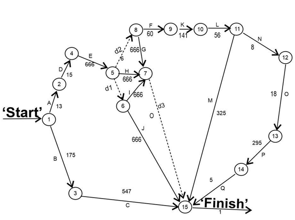
The appendix, which was produced using freely accessible data from [28, 29, 30]’s research work, offers an illustration of this. The most likely time, the optimistic and pessimistic timings, and the duration of the activity could be described in hourly, daily, weekly, monthly, or quarterly intervals, as well as quarterly or annually, depending on how long it takes. The proposed conceptual framework was verified. This estimate, which consists of three time estimations, is referred to as the most probable time (MLT), pessimistic time (PST), and optimistic time (OPT). The data is shown as a network diagram in Figure 1, where the numbers on the arrows correspond to the figures utilized in the study. Version 2.00 of the TORA optimization program was used to perform PERT calculations.
Figure: Figure 1 depicts a project from beginning to end. While nodes represent the completion of an activity, arrows represent the task. The arrows indicate how long each activity will take to complete. Displays that have dotted lines are a task that cannot be completed. Creating a network model of the project, like the one in Figure 1, in which each arc stands for an action and each node for an event, is the first step in using PERT. The activity time is used as a random variable in the PERT model. The project manager needs to estimate each of the following three things: a calculation of the activity’s maximum time frame, as represented by (OPT). Estimation of the activity’s duration under the most difficult conditions is shown by (PST). The value that represents the most likely length of the activity is represented by (MLT). Estimating the length of jobs and the likelihood that they will be completed on time, which might be arbitrary and wrong. This might result in either an overestimate or underestimate of the time required to finish a project.
Anderson Darling Normality Test
States that the Anderson-Darling test is employed to the normal distribution was used to choose the data sample [31].
Anderson-Darling Test Statistic: The Anderson-Darling test (ADT) is employed to examine whether a given data sample originates from a population characterized by a particular distribution. It is an adaptation of Cramer-Von Misses (CVM) test and distinguishes itself by placing greater emphasis on the tails than the CVM test. In contrast to the distribution- free nature of the CVM test, the AD test incorporates a predefined hypothesized distribution in its computations of critical values. The AD test statistic is given by [24, 25, 32]
1 2 1 1 2 2 1 log 1 0.75 2.25 1
( ) ( ) { }
$$ A = \left\{- \left(1 + \frac {0 . 7 5}{n} + \frac {2 . 2 5}{n ^ {2}}\right) \left[ \frac {\sum_ {i = 1} ^ {n} \left\{\left(2 i - 1\right) \log \left[ z _ {i} \left(1 - z _ {n + 1 - i}\right) \right] \right\}}{n} + n \right] \right\} ^ {\frac {1}{2}} $$ n i n i i i z z A n n n n Where:
$$ z _ {i} = \phi \frac {y - \mu}{\sigma} $$
ϕ(.) = Distribution functions of a standard normal variable. n = Sample size Kolmogorov Smirnov Normality Test The Kolmogorov-Smirnov test is a statistical test that is used to confirm if a sample is representative of a specific distribution, like the normal distribution. Since it is non-parametric, it does not assume anything about the distribution of the data [27]. The sample data for the Kolmogorov-Smirnov test should originate from a specified distribution, like the normal distribution, according to the null hypothesis. An alternative scenario could be that the sample data do not accurately reflect the given distribution [26].
Kolmogorov Smirnov Test Statistic: The largest absolute difference between the cumulative distribution function (CDF) of the sample data and the CDF of the given distribution serves as the test statistic in the Kolmogorov-Smirnov test. The following formula is used to determine the test statistic D $$ D = \max | F (x) - S (x) | $$ Where: D = Kolmogorov Smirnov test statistic F (x) = Cumulative distribution function (CDF) S(x) = Empirical distribution function (ECDF)
Shapiro Wilks Normality Test
A statistical test called the Shapiro-wilk test is used to discover whether a dataset has a normal distribution. Martin Wilk and Samuel Shapiro created it in 1965 [22]. The community from which the sample is drawn must have a normally distributed population in order for the test to be considered valid. To evaluate the significance of the deviation from normality, the test gives a p-value. The Shapiro-Wilk test is frequently used to determine whether the collected data conforms to a normal distribution, a prevalent assumption in many statistical analyses, in a variety of disciplines including biology, social sciences, engineering, and finance. To assess the normality assumption, it is important to keep in mind that while the test is helpful, it is not infallible, so it should be used in conjunction with other tests and visualizations.
The Shapiro Wilk test is more appropriate method for small sample sizes ($i_{50}$ samples) although it can also be handling on larger sample size while.
Shapiro Test Statistic: W stands for the Shapiro-wilk test statistic, which is displayed below.
$$W = \frac{\left( \sum a_i x_i \right)^2}{\sum \left( x_i - \bar{x} \right)^2}$$
- Where:
- $W = W$ is the Shapiro-Wilk test statistic
- $a_i$ = Coefficients that depend on the sample size and are obtained from pre-calculated tables
- $x_i$ = Ordered sample values
- $\bar{x}$ = Sample Mean
- The test statistic $W$ ranges from 0 to 1, with values closer to 1 indicating that the sample is more likely to have been drawn from a normally distributed population. The p-value is then calculated based on the value of $W$ and the sample size.
Skewness Normality Test
To determine whether an estimated time is normal, one can utilize the Pearson index. Using Pearson’s Index (PI) of skewness can be verified. The equation is
$$PI = \frac{3(\bar{x} - \text{median})}{s}$$
- Where
- $\bar{x}$ = sample mean
- $s$ = sample standard deviation
If Pearson Index of:
1. Skewness = 0: The distribution is entirely symmetrical if the skewness coefficient is zero. This suggests that the distribution is bell-shaped, just like the normal distribution, and that the mean, median, and mode are all equal.
2. Skewness > 0: The distribution has a longer or fatter tail on the right (or positive) side than the left, as indicated by a positive skewness coefficient. Stated otherwise, there is a rightward bias in the distribution. In these situations, the data is concentrated on the left side of the distribution and the mean is usually higher than the median.
3. Skewness < 0: A distribution with a left (or negative) tail that is longer or fatter than the right is said to have a negative skewness coefficient. There is a leftward skew in the distribution. In this instance, the data is concentrated on the right side of the distribution, and the mean is usually lower than the median.
Check for Outliers
Any data point that considerably deviates from the observation is considered outliers [23]. Gather the data set first and then arrange it in ascending order. Next, we determine the data’s 25th and 75th percentiles. The difference between the 75th and 25th percentile is then used to construct the interquartile range, or IQR. We determine the lower and upper outlier thresholds. Then, if there are any outliers, we find any data values that are either smaller than the lower threshold or larger than the upper threshold and print them.
Any predicted result that falls outside of the normal range (25th percentile minus 1.5 time’s interquartile range) or exceeds the normal range (75th percentile plus 1.5 times interquartile range) is referred to as an outlier. There are no outliers in any of the observed estimations as a result. Otherwise, you must throw the estimates away and create a new one until they are no outlier. Table 4 shows the outlier identification summary results.
Result
Result and Interpretations for Anderson-Darling test
The results of the Anderson-Darling test for normality are shown in Table 1. The alternative hypothesis contends that the data are not normal, while the null hypothesis maintains that the data come from a normal distribution. Since the most probable time (MLT) p-value is 0.4389, over the significance level of 0.05, the Anderson Darling test does not rule out normalcy. The results likewise held true for estimates of pessimistic time (PST) and optimistic time (OPT); the corresponding p-values for PST and OPT were
0.2037 and 0.2606, respectively, both above the significance level of 0.05. Therefore, it is believed that the data is regularly distributed. R software, version 4.3.3, was used for all computations [33]. Version 2.00 of the TORA optimization program was used to perform PERT calculations.
| STATISTIC | MLT | VARIABLE PST | OPT |
|---|---|---|---|
| A | 0.3454 | 0.4757 | 0.4347 |
| P - Value | 0.4389 | 0.2037 | 0.2606 |
| D | 0.16585 | 0.18654 | 0.19638 |
| P - Value | 0.8038 | 0.6736 | 0.6094 |
| W | 0.94186 | 0.92808 | 0.92518 |
| P - Value | 0.4063 | 0.2554 | 0.231 |
| Pearson Index | 0.4974556 | 1.065967 | 0.3656811 |
| Mean | 15.26667 | 17.6 | 12.86667 |
| Median | 14 | 15 | 12 |
| σ | 7.638873 | 7.317298 | 7.11002 |
| Q1 | 10 | 12.5 | 9 |
| Q3 | 19.5 | 24 | 15.5 |
| IQR | 9.5 | 11.5 | 6.5 |
| (1.5)IQR | 14.25 | 17.25 | 9.75 |
| Q1 - (1.5)IQR | -4.25 | -4.75 | -0.75 |
| Q3 + (1.5) IQR | 33.75 | 41.25 | 25.25 |
| Minimum | 5 | 7 | 3 |
| Maximum | 32 | 30 | 30 |
Table 1: Summary Result.
Result and Interpretations for Kolmogorov- Smirnov Test
The Kolmogorov-Smirnov test compares the alternative hypothesis, which states that the data do not originate from a normal distribution, to the null hypothesis, which states that a set of data does. Table 1 displays the computation results using the Kolmogrov test statistic. When the number of samples is more than fifty, the Kolmogorov-Smirnov test is utilized. The data are from a regularly distributed population, as per the null hypothesis. When P is greater than 0.05, the null hypothesis is accepted and the data are referred to as normally distributed. The results indicate that the most probable time (MLT) is 0.8038, the optimistic time (OPT) is 0.6094, and the pessimistic time (PST) is 0.6736, all of which are more than 0.05. Table 1 below displays the summary results for the Kolmogorov-Smirnov test.
Result and Interpretations for Shapiro-Wilk Test
Although the Shapiro-Wilk test is better appropriate for smaller sample sizes (less than 50 samples), it can be used with larger sample sizes as well. The null hypothesis states that the data are from a normally distributed population. P larger than 0.05 denotes a normal distribution of the data and the acceptance of the null hypothesis. Here, a sample size of 15 is employed. R version 4.3.3, the statistical package, was used for all computations [34]. The null hypothesis is accepted and it is concluded that the data is normally distributed because the most likely time (MLT) P value is 0.4063, which is greater than 0.05, the pessimistic time (PST) P value is 0.2554, which is also greater than 0.05, and the optimistic time (OPT) P value is 0.2310, which is greater than 0.05. Table 1 below displays the summary results for the Shapiro-Wilks test.
Results and Interpretation for Skewness
Consequences of skewness derived from Pearson Index are as follows:
- Measures of central tendency like the mean, median and mode are impacted by skewness in their interpretation. The mean is drawn towards the lower values in negatively skewed distributions and the higher values in positively skewed distributions.
- Skewness has an impact on how statistical analyses operate and are interpreted. For instance, skewness in parametric statistics can lead to assumptions of normalcy being broken, which can result in skewed estimates or inaccurate conclusions.
- In a variety of disciplines, including risk management, economics, and finance, an understanding of skewness is crucial.
In particular, whether dealing with financial assets or project outcomes, skewed distributions can have an impact on risk assessment and decision-making processes. Before using certain statistical procedures, skewed data may need to be transformed in order to establish normalcy or stabilize variance. The logarithmic, square root, and inverse transformations are examples of common transformations.
There are various repercussions when outliers in a dataset are not detected: 1. Statistics like the mean and standard deviation can be severely distorted by outliers. Outliers can cause skewed estimates of central tendency and dispersion, which can impact how the data is interpreted overall, if they are not appropriately recognized and managed. 2. Data visualizations like scatter plots, box plots, and histograms can be distorted by outliers. When
outliers are overlooked, the data distribution may be represented visually in a way that is misleading and makes it challenging to see the underlying patterns and relationships within the dataset. 3. Predictive models’ parameters may be impacted by outliers, which could result in incorrect predictions. When applied to new data, models trained on outlier- filled data may perform badly because they may identify noise or anomalies instead of real patterns in the data. 4. True links and patterns can be more difficult to identify when there are outliers in the data due to the increased unpredictability. Increased am- biguity in the analytical and decision-making processes may result from this. 5. Algorithms and methods used in data analysis can become less effective due to outliers. It frequently takes more time and processing power to identify and handle outliers, especially in large datasets. 6. In some situations, including financial analysis or quality control, outliers might constitute serious irregularities or hazards that require attention. Underestimating these risks due to a failure to recognize outliers may result in monetary losses or problems with quality. 7. Many statistical techniques rely on the assumption that the data are either outlier-free or regularly distributed. These presumptions may be broken by failing to spot outliers, which could result in erroneous findings or improper use of statistical tests.
Sensitivity Analyses
Like any statistical or machine learning technique, outlier detection techniques have their limits. Here are a few typical ones:
- Numerous techniques for detecting outliers presume a specific data distribution, like the normal distribution. The procedures might not work effectively if the data doesn’t match certain presumptions.
- A lot of outlier identification methods have parameters, such the threshold for what counts as an outlier that needs to be adjusted. These parameters may be sensitive, and the values selected for them can have a big impact on the outcome.
- The computational cost of certain outlier detection techniques can be high, particularly when working with huge datasets. The time and memory requirements of these technologies may become unaffordable as the dataset grows.
- The definition of an outlier can vary greatly depending on the context; a data point that is deemed an outlier in one context might not be in another and outlier identification techniques could not always account for this context dependence.
- It may be difficult for outlier identification algorithms to discern between data noise and outliers. False positives can occur when noise is mistaken for outliers.
- When dealing with data that has several clusters or modes, outlier detection techniques cannot work well. They might not be able to efficiently identify outliers within each mode or cluster.
- Outlier detection techniques may have trouble correctly identifying outliers in datasets where they are uncommon. This is especially true for density estimation-based approaches, which have a tendency to give outliers low probabilities.
- It’s possible that outlier detection techniques won’t adjust well to gradual shifts in the data distribution. When the data changes, a procedure that performs well at first could become less effective.
- Some techniques for identifying outliers don’t explain much about why a specific data point is deemed to be an outlier. It could be difficult to comprehend and have faith in the results due to this lack of interpretability.
- The more dimensional the data, the more difficult it is to identify outliers.
The curse of dimensionality causes many traditional methods to fail when dealing with high- dimensional data.
Discussion
A project management tool called the Project Evaluation Review Technique (PERT) is used to plan, arrange, and coordinate work inside a project. Projects with a high degree of unpredictability and complexity benefit most from it.
Future Implication on Project
PERT has various real-world applications.
- Through the estimation of job completion times and the identification of the critical path the longest path through the project network PERT assists in scheduling the project. Project managers may now set reasonable timelines and distribute resources more effectively.
- PERT helps with resource allocation by determining dependencies be- tween tasks and estimating the amount of time needed for each activity. Project managers have the ability to distribute resources, including labour, supplies and machinery, based on the demands of individual tasks and the project schedule.
- PERT takes uncertainty into account by employing three time estimates for every task: most likely, pessimistic, and optimistic. This aids in recognizing and controlling risks related to task duration. Project managers can determine the possibility of fulfilling project deadlines and take proactive steps to reduce risks by examining the range of time estimates.
- PERT offers a framework for monitoring project progress through the comparison of expected and actual job completion times. Early detection of schedule deviations enables project managers to take remedial measures, such as reassigning resources or changing job priorities.
- PERT facilitates collaboration and communication amongst members of a project team by outlining responsibilities, deadlines, and dependencies in detail. It encourages teamwork and guarantees that all project participants are aware of their respective roles and responsibilities.
- PERT makes performance evaluation easier by giving a foundation for contrasting actual and projected project performance. This makes it possible for project managers to evaluate the efficacy and efficiency of the project’s execution and pinpoint areas that need improvement for subsequent initiatives.
- PERT gives project manager’s useful data to help them make decisions about things like adding more resources to important tasks or modifying project deadlines.
It makes it possible to make well informed decisions based on impartial facts and research.
Real Time Case Study
Project evaluation review approaches are widely employed in several industries to evaluate the advancement and efficacy of projects. Here are a few examples of current case studies where these strategies were effectively applied Construction Project Management: Case Study: To evaluate the status of a high rise building construction project, a major construction business used project evaluation review procedures. Through the application of methodologies such as Earned Value Management (EVM) and Critical Path Method (CPM), the project managers were able to monitor the project’s cost performance, schedule adherence, and early identification of possible risks. Frequent project review meetings made it easier to spot bottlenecks and move quickly to address them, which allowed the project to be successfully completed on schedule and under budget. Case Study on: Information Technology (IT) Project Management Project assessment review procedures were used by a software development company to oversee the creation of a new software application. By using methods such as sprint reviews and agile approaches, the project team was able to regularly assess the project’s progress. They found areas for improvement and made the required changes to the project plan by holding regular retrospectives. This method allowed for quick adjustments to requirements that changed and guaranteed the high-quality software product was delivered on schedule. Healthcare Project Management: Case Study: To improve its healthcare information system, a hospital used project evaluation and review methodologies. The project team tracked any deviations from the project plan and tracked the implementation progress using tools like milestone track- ing and Key Performance Indicators (KPIs). Stakeholders participated in regular review sessions, which aided in resolving problems quickly and guaranteeing conformity with corporate objectives. Consequently, the new information system was successfully implemented, improving patient care and operational effectiveness. Case Study on Manufacturing Project Management: To introduce a new electric vehicle production line, an automotive manufacturing business used project assessment review methodologies. The project managers monitored the status of different activities and resource consumption by using tools such as Gantt charts and resource allocation analysis. Periodic performance evaluations facilitated the identification of possible setbacks and efficient resource allocation to achieve production objectives. As a result, the new production line was introduced on time and helped the business achieve its strategic goals of innovation and sustainability. Project Management for Infrastructure Development: A Case Study a government organization supervising the building of a new transportation infrastructure project, like a bridge or roadway, used project assessment review methodologies. Project managers tracked project performance and found any hazards that might have an impact on project delivery by us- ing strategies like risk analysis and Performance Measurement Baseline (PMB). Frequent project audits and reviews made sure that safety regulations and legal requirements were followed. The infrastructure project’s successful completion increased the area’s transportation connectivity and sparked economic growth.
Conclusion
The project evaluation review technique (PERT), a planning tool utilized in project management, is given a straightforward addition in this research work. The strategy depends on an assessment of the activity’s time and likelihood of timely completion, which may be arbitrary and wrong. This can cause some- one to overestimate or underestimate how long it will take to complete a task. Information is gathered for each action regarding the task’s most likely completion time, the task’s completion time under the worst scenario, and the task’s completion time under the best scenario. This study carried out the investigation using published data sets. Given that the P-values are greater than the significance level of 0.05, the results of the Anderson-Darling Test for Normality show that both variables have a normal distribution. P-values above the significance level of 0.05 in the Kolmogorov-Siminov Test results for normality show that both variables had a normal distribution. The Shapiro- Wilks Test findings for normality show that both variables had a normal distribution because the P-values were greater than the significance level of 0.05. In order to determine the normality of the data set, we employed the Kolmogorov-
smirnov test, the Shapiro-wilks test, the skewness test, and the check for outliers. As P-values are greater than 0.05, the Kolmogorov-Smirnov test for normality reveals that all variables were normally distributed. The most likely time, the most pessimistic time, and the most optimistic time are both normally distributed, according to the Shapiro-Wilks test results. With the exception of the most optimistic time prediction, which shows skewness to the right, all the variables indicate that the Pearson Index is not considerably skewed. All of the observed estimations lack outliers. This study opened up new possibilities for project management and control, and also improved the usefulness of existing planning tools.
The results of the Kolmogorov-Siminov test likewise indicate that all three of the variables are normally distributed, supporting the findings of the Anderson Darling test that all tree variables are normally distributed. Normalcy has also been determined by the Shapiro-Wilks test. There are numerous actions that must be completed as part of a project. Every activity has a start time and an end time. These estimates were made at random based on the expert’s knowledge and discretion. The most probable, pessimistic, and optimistic estimates are the three categories. However, because these estimations are made subjectively, they are vulnerable to under- or overestimation. The fact that they are regularly distributed is demonstrated by the three estimates (i.e., pessimistic, most likely, and optimistic). Otherwise, you must throw the estimates away and create a new one until they are distributed normally. The purpose of the article is to remove any uncertainty from activity time estimations made using project assessment review technique. The unique method will undoubtedly ensure the impartiality of the activity time calculation.
In conclusion, the Pearson index of skewness influences data interpretation, statistical analysis, risk assessment, and decision making across a range of fields by offering insightful information about the asymmetry and shape of a distribution.
In general, failing to recognize outliers might jeopardize the accuracy and dependability of data analysis findings, sometimes resulting in erroneous judgments and conclusions. For this reason, in every data analysis process, it is crucial to thoroughly detect and handle outliers. When applying outlier detection techniques, it’s critical to be aware of these limitations and carefully assess whether the techniques are suitable for the given dataset and issue area. Some of these restrictions can also be lessened by combining several techniques or directing the outlier detection process with domain expertise.
Ultimately, by offering a methodical approach to project management, in- creasing efficiency, lowering risks, and guaranteeing project success, PERT aids in improving project planning, execution, and control. These case studies show how project assessment review procedures work well across a range of industries and emphasize how important they are to successfully completing projects on schedule, under budget, and with acceptable quality standards.
References
-
Malcom DG, Roseboom JH, Clark CE, Fazer W (1959) Application of a Technique for Program Development and Evaluation. Operations Research 7(5): 557-685.
-
Grubbs FE (1962) Attempts to Validate Certain PERT Statistics or Picking on PERT. Operations Research 10(6): 912-915.
-
Moder JJ, Phillips CR, Davis EW (1983) Project Management with CPM, PERT and Precedence Diagramming. Van Nostrand Reinhold, pp: 389.
-
Badiru AB (1991) Simulation approach to PERT Network Analysis. Simulation 57(4): 245-255.
-
Crimmon KR, Ryavec CA (1964) Analytical Study of the PERT Assumptions. Operations Research 12(1): 16-37.
-
Bride WJJ, Clelland CW (1967) Pert and the Beta Distribution. IEEE Transactions on Engineering Management NJ 14(14): 166-169.
-
Wayne D, Cottrell PE (1999) Simplified Program Evaluation and Review Technique (pert). Journal of Construction Engineering and Management 125(1): 16- 22.
-
AbouRizk SM, Halpin DW (1992) Statistical Properties of Construction Duration Data. Journal of Construction Management 118(3): 525-544.
-
AbouRizk SM, Halpin DW (1994) Fitting Beta Distribution based on Sample Data. Journal of Construction Management 120(2): 288-305.
-
Callahan MT, Quackenbush DG, Rowings JE (1992) Construction Project Scheduling. In 7th (Edn.), Graw H, USA.
-
Fulkerson DR (1962) Expected Critical Paths Lengths in PERT Networks. Operations Research 10(6): 808-817.
-
Van RM (1963) Monte Carlo Methods and the PERT Problem. Operations Research 11(5): 839-860.
-
Dodin B (1984) Determining the K most Critical Paths in PERT Networks. Operations Research 32(4): 859-877.
-
Bandopadhyay S, Sundararajan A (1987) Simulation of a Long Wall Development Extraction Network. CIM Bull 903(80): 62-70.
-
Lindsey JH (1972) An Estimate of Expected Critical Path Length in PERT Networks. Operations Research 20(4): 800-812.
-
Hartley HO, Wortham AWA (1996) Statistical theory for PERT Critical Path Analysis. Management Science 12(10): B391-C229.
-
Robillard P, Trahan M (1977) The Completion Time of PERT Network. Operations Research 25(1): 15-29.
-
Kamburowski J (1985) Normally distributed activity durations in PERT networks. Journal of Operations Research Society 36(11): 1051-1057.
-
Anklesaria KP, Drezner ZA (1986) Multivariate approach to Estimating the Completion time for PERT networks. Journal of Operations Research Society 37(8): 811-815.
-
Sculli D, Shum YW (1991) An Approximate Solution to PERT Problem. Computer and Mathematics Applications 21(8): 1-7.
-
Crandall KC (1976) Probabilistic Time Scheduling. Journal of Construction Division 102(3): 415-423.
-
Nornadiah MR, Yap BW (2011) Power Comparisons of Shapiro-Wilk, Kolmogorov-Smirnov, Lilliefors and Anderson-Darling tests. Journal of Statistical Modeling and Analytics 2(1): 21-33.
-
Bluman AG (2009) Elementary Statistics: A Step by Step Approach. 7th (Edn.), 1221 Avenue of the Americas, New York, USA.
-
Afeez BM, Maxwell O, Otekunrin OA, Happiness O (2016) Selection and Validation of Comparative Study of Normality Test. American Journal of Mathematics and Statistics 8(6): 190-201.
-
Das KR, Imon AHM (2016) A Brief Review of Tests for Normality. American Journal of Theoretical and Applied Statistics 5(1): 5-12.
-
Simard R, Lecuyer P (2011) Computing the Two-Sided Kolmogorov Smirnov Distribution. Journal of Statistical Software 39(11): 1-18.
-
(2021) Kolmogorov Smirnov Goodness of fit test. Technical Report. National Institute of Standards and Technology NIST.
-
Cynthia OU (2020) Implementation of Project Evaluation and Review Technique (PERT) and Critical Path Method (CPM): A Comparative Study. International Journal of Industrial and Operations Research 3(1): 1-9.
-
Aliyu AM (2013) Project Management using CPM: A Pragmatic Application. Global Journal of Pure and Applied Sciences 18(3-4): 197-206.
-
Maidamisa AA (2017) Comparative Analysis of Activity Duration in Project Management. International Journal of Business and Management 5(12): 158-162.
-
Stephens MA (1974) EDF Statistics for Goodness of Fit and Some Comparisons. Journal of the American Statistical Association 69(374): 730-737.
-
Baghban A, Younespour S, Jambarsang S, Yousefi M, Zayeri F, et al. (2013) How to Test Normality Distribution for a Variable: A Real Example and A Simulation Study. Journal of Paramedical Sciences 4(1): 73-77.
-
Michel NJ, Kevin K, Severin B, Zoro B (2021) Genetic Diversity of Taro Landraces from Cote d Ivoire Based on Qualitative Traits of Leaves. Agricultural Sciences 12: 1-12.
-
John MC (2020) S, R and Data Science. The R Journal 12(1): 462-476.
- Revolutionizing Property Measurement Through Artificial Intelligence: The Journey of PropertyMeasure.ai
- AI Infused Business Model Innovation for Competitive Advantage in the Era of Big Data and Digital Transformation
- Use of CPM/PERT in the Effort to Eradicate Polio
- Integrated Multimodal Deep Learning Framework for Early Detection of Mouth Cancer Using CT Imaging and Clinical Symptom Analysis
- Artificial Intelligence in Medical Robotics and Assistance: An Overview
- Server Migration with Multipath-QUIC