The Difference between the Chemical Short Range Orders of Binary Liquid Alloys Using Different Models
The thermodynamic models based on cluster of two and four atoms were considered to obtain the thermodynamic properties of liquid binary alloys. The four liquid alloys are candidates of homo-coordination / self-coordination. The values of chemical short range order, Concentration fluctuation and excess stability functions and the differences in models computed for Cu-Pb, Li-Mg, Cd-Ga and Bi-Cd binary liquid alloys are presented.
Introduction
The electron microscopy and x-ray diffraction experiments are very useful tool to obtaining the structural information and thermodynamic properties of binary liquid alloys Singh [1]. In most cases, obtaining the experimental data needed for the calculation of specific thermodynamic properties are really available (except in some uncommon cases where the experimental data for some alloys may be difficult to obtain due to cumbersome task involved and experimental complexities). In principle, the chemical short range order ( )has connection with the Concentration- Concentration Fluctuation in the long wave length limit (Scc (0)). The Scc(0) can be experimentally determined from the knowledge of concentration-concentration partial structural factor, Scc (q), and the number-number partial structural factor SNN (q) Bhatia, et al. [2]. However, these structures are not easily measurable in most diffraction experiments. Hence is usually computed when experimental values are not available. Additionally, a direct experimental determination of Scc (0) is often avoided due to great deal of task often involved [3]. For this reason the options of thermodynamic models which have been used were employed and juxtaposed.
The focus of this study, therefore, is to compute the excess stability functions of two binary liquid alloys via Statistical Mechanical Model (SMM) [4], Quasi-Lattice Model (QLM), Two and Four Atoms Cluster models (TACM and FACM) [5]. The results comparisons would be made thereafter to ascertain to what extent it is safe to consider these approaches.as the two options serves as alternatives when information on concentration-concentration fluctuation is attached.
In doing the aforementioned, we applied these models to Cu-Pb, Li-Mg, Cd-Ga and Bi-Cd liquid alloys [6, 7] for the qualitative investigation of their thermodynamic properties. Ordering energy values determined from Scc (0) are recorded in Table 1. Programs were inscribed to generate data for thermodynamic expressions as functions of concentration, c, using ordering energy values, w, coordination number, Z, Boltzmann constant, K and temperature, T presented in Table 1.
| Alloy | Temperature(oK) | Z | W (eV) 1 | W (eV) 2 | ∆W=W -W (eV) (QLM-SMM) 2 1 |
|---|---|---|---|---|---|
| Cu-Pb | 1473 | 10 | 0.2289 (QLM) | 0.2264 (SMM) | 0.0025 |
| Li-Mg | 887 | 10 | -0.0764 (QLM) | -0.0764 (SMM) | 0.0000 |
| Cd-Ga | 700 | 10 | 0.1133 (TACM) | 0.1145 (FACM) | 0.0012 |
| Bi-Cd | 773 | 10 | 0.0210 (TACM) | 0.0213 (FACM) | 0.0003 |
Table 1: Ordering energy (w) in eV of binary alloys.
Theory
The determination of ordering energy (w) or interchange energy can be linked to the calculation of the Chemical Short Range Order ( 1 α ) of binary liquid alloys. The variation of this quantity with composition is informative [8]. Thermodynamically, the relationship between short range order parameter 1 α and other thermodynamic properties had been sighted in the literature Khanna, et al. [9, 10]. Moreover, between w and 1 α and other properties they are given below. The following thermodynamic expressions are from different Models.
Expressions for Chemical Short Range Order (SMM)
$$ \left(1 + \frac {\alpha_ {1}}{c \left(1 - c\right) \left(1 - \alpha_ {1}\right) ^ {2}}\right) = \exp \left(\frac {2 w}{z K _ {B} T}\right) $$
2 1 exp 1 1 B
α w zK T c c
(1)
1 2 1 ( )( )
α Z is the coordination number for the first shell, w is the ordering energy, K is the Boltzmann constant, T is the temperature, c is concentration of atom A and 1-c is the concentration of atom B.
Expressions for Chemical Short Range Order (QLM)
( ) ( ) ( ) 1 2 1 1 exp 2 1 1 B C C w Z K T α (2)
$$ \frac {\alpha_ {1}}{\left(1 - \alpha_ {1}\right) ^ {2}} = C \left(1 - C\right) \left(\exp \left(2 w / Z K _ {B} T\right) - 1\right) $$ ( )
Results
Concentration-Concentration Fluctuation in the Long Wavelength Limit (TACM &FACM) ( ) (1 ) 0 (1 ( )(1 ) 2 c c Scc Z β β $$ ) = \frac {c (1 - c)}{(1 + \left(\frac {Z}{2 \beta}\right)) (1 - \beta)} $$ (3) $$ \text {W h e r e} \eta = \exp (w / Z K T) \tag {4} $$ and Z is the coordination number for the first shell, w is the ordering energy, K is the Boltzmann constant, T is the temperature, c is concentration of atom A and 1-c is the concentration of atom B.
$$ \mathrm {w h e r e} \beta = (1 + 4 c (1 - c) [ (\eta) (\eta) - 1 ]) ^ {0. 5} \tag {5} $$ η and β are thermodynamic parameters which are interwoven Excess Stability Function (ES) (TACM &FACM) $$ E S = \frac {R T}{S c c (0)} - \frac {R T}{c (1 - c)} [ 6 ] $$ Ideal Concentration-Concentration Fluctuation in the Long Wavelength Limit $$ S c c _ {c c} ^ {i d} (0) = c (1 - c) \tag {7} $$
R is molar gas constant.
(0) (1 ) id
| Ccu | α QLM 1 | α 1SMM | α 1Difference |
|---|---|---|---|
| 0.0 | 0.0000 | 0.0000 | 0.0000 |
| 0.1 | 0.0290 | 0.0363 | 0.0730 |
| 0.2 | 0.0500 | 0.0612 | 0.0112 |
| 0.3 | 0.0640 | 0.0776 | 0.0136 |
| 0.4 | 0.0720 | 0.0869 | 0.0149 |
| 0.5 | 0.0740 | 0.0899 | 0.0159 |
| 0.6 | 0.0720 | 0.0869 | 0.0146 |
| 0.7 | 0.0640 | 0.0776 | 0.0136 |
| 0.8 | 0.0500 | 0.0612 | 0.0112 |
| 0.9 | 0.0290 | 0.0363 | 0.0073 |
| 1.0 | 0.0000 | 0.0000 | 0.0000 |
| CLi | α QLM 1 | α SMM 1 | α Difference 1 |
| 0.0 | 0.000 | 0.000 | 0.0000 |
| 0.1 | -0.017 | -0.017 | 0.0000 |
| 0.2 | -0.0352 | -0.0353 | 0.0001 |
| 0.3 | -0.0455 | -0.0455 | 0.0000 |
| 0.4 | -0.0497 | -0.0497 | 0.0000 |
| 0.5 | -0.0496 | -0.0496 | 0.0000 |
| 0.6 | -0.048 | -0.048 | 0.0000 |
| 0.7 | -0.0453 | -0.0453 | 0.0000 |
| 0.8 | -0.0437 | 0.0437 | 0.0000 |
| 0.9 | -0.0411 | -0.0411 | 0.0000 |
| 1.0 | 0.0000 | 0.0000 | 0.0000 |
Table 2: Calculated QLM and SMM for 1 α of Cu-Pb alloy Ccu is the concentration of copper in the alloy at 1473 OK.
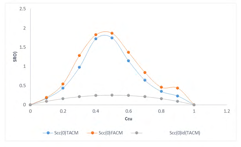
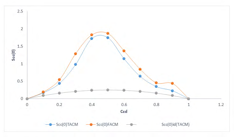
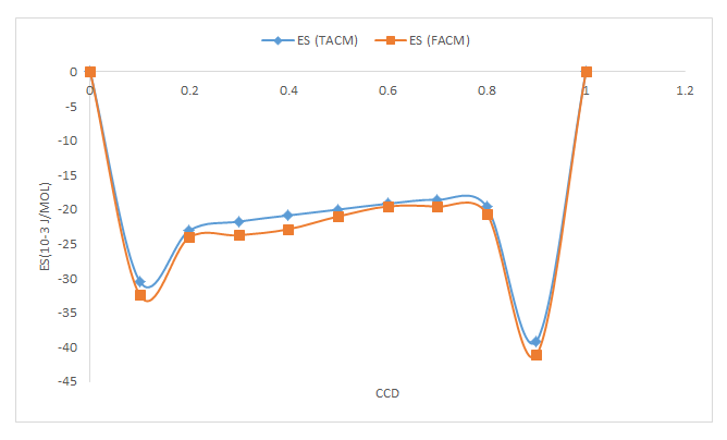
| Ccd | Scc(0) TACM | Scc(0) FACM | Scc(0)Id | ES (TACM) ( 10-3 J/ mol) | ES (FACM) ( 10-3 J/ mol) | ES (FACM-TACM) ( 10-3 J/ mol) |
|---|---|---|---|---|---|---|
| 0.0 | 0.00 | 0.00 | 0.00 | 0.0000 | 0.0000 | 0.000 |
| 0.1 | 0.17 | 0.19 | 0.09 | -30.4301 | -32.4351 | -0.005 |
| 0.2 | 0.437 | 0.543 | 0.16 | -23.0545 | -24.0565 | -0.002 |
| 0.3 | 0.976 | 1.286 | 0.21 | -21.7494 | -23.7523 | -0.0171 |
| 0.4 | 1.718 | 1.823 | 0.24 | -20.8615 | -22.8643 | -0.0028 |
| 0.5 | 1.745 | 1.864 | 0.25 | -20.006 | -21.0071 | -0.0011 |
| 0.6 | 1.143 | 1.367 | 0.24 | -19.158 | -19.5597 | -0.0017 |
| 0.7 | 0.638 | 0.842 | 0.21 | -18.5918 | -19.5936 | -0.0018 |
| 0.8 | 0.347 | 0.456 | 0.16 | -19.6044 | -20.6056 | -0.0016 |
| 0.9 | 0.228 | 0.435 | 0.09 | -39.139 | -41.141 | -0.002 |
| 1.0 | 0.000 | 0,0000 | 0.00 | 0.000 | 0.000 | 0.000 |
Table 3: Calculated TACM and FACM for Scc(0) and ES of Cd-Ga alloy Ccd is the concentration of cadmium in the alloy at 700 OK.
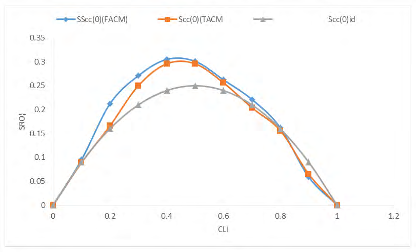
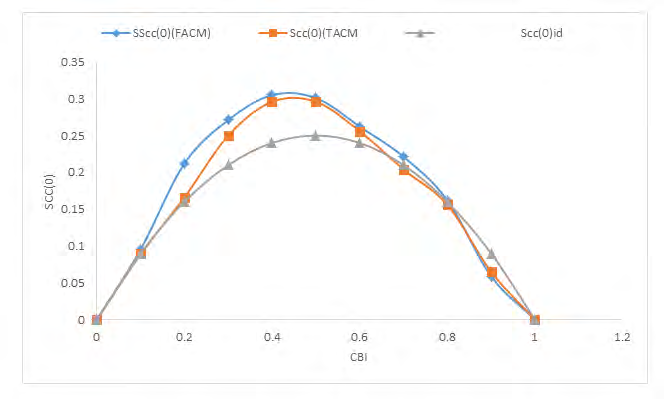
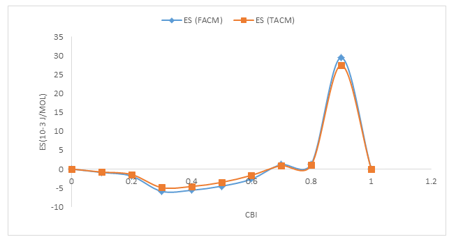
| Ccd | Scc(0) TACM | Scc(0) FACM | Scc(0)Id | ES (TACM) ( 10-3 J/mol) | ES (FACM) (10-3 J/mol) | ES (FACM-TACM) ( 10-3 J/mol) |
|---|---|---|---|---|---|---|
| 0.0 | 0.000 | 0.0000 | 0.00 | 0.0000 | 0.0000 | 0.00 |
| 0.1 | 0.089 | 0.0953 | 0.09 | -0.8023 | -0.9043 | -0.002 |
| 0.2 | 0.166 | 0.2121 | 0.16 | -1.4516 | -1.8752 | -0.0006 |
| 0.3 | 0.25 | 0.2711 | 0.21 | -4.8961 | -5.8978 | -0.0017 |
| 0.4 | 0.296 | 0.3051 | 0.24 | -4.6168 | -5.6176 | -0.0008 |
| 0.5 | 0.296 | 0.3011 | 0.25 | -3.5459 | -4.5463 | -0.006 |
| 0.6 | 0.256 | 0.2622 | 0.24 | -1.6736 | -2.6745 | -0.0019 |
| 0.7 | 0.204 | 0.2213 | 0.21 | 0.9004 | 1.2013 | -0.0009 |
| 0.8 | 0.156 | 0.1622 | 0.16 | 1.031 | 1.3332 | -0.0022 |
| 0.9 | 0.065 | 0.0589 | 0.09 | 27.4645 | 29.4656 | -0.002 |
| 1.0 | 0.000 | 0.0000 | 0.00 | 0.0000 | 0.0000 | 0.000 |
Table 4: Calculated TACM and FACM for Scc(0) and ES of Cd-Ga alloy Ccd is the concentration of cadmium in the alloy at 700 OK.
Discussion
Figures 1 & 2 displayed the relationship between the SROs and the concentrations of copper and lithium in their liquid phase. The figures portray homo-coordination in the nearest neigbour shell. The atomic distributions signifies like-atoms pairing in the neigbourhood shells. Figures 3 & 5 shows the plots of concentration-concentration fluctuation Scc (0) against concentration of element for Cd-Ga, and Bi- Cd liquid alloys at their melting temperatures. The Scc(0) of these alloys increases initially to a maximum (owing to the charge transfer between neighboring atoms) within the entire concentration range with distinct peaks at Ccd = 0.5 and CBi = 0.4, and, the remaining liquid alloy has some depression at the right side of the curve (owing to chemical alternation of positive and negative charges with length scale approximately twice the nearest neighbor distance). In Figure 3, the calculated Scc (0) is in not perfect agreement with ideal solution values This is because the is a near cancellation of the ionic potentials wile at large distances ionic potentials was screened. Figure 3 & 5 also, have their calculated values for Scc(0) of Cd-Ga and Bi-Cd above the ideal solution values which are in support of homocoordination or self coordination.
Figures 4 & 6 shows the plots of excess stability function versus concentration of element. The display in Figure 4 shows an initial decease in curve to a minimum (possibly when the disordered potential is too large) with a corresponding gradual increase and some fluctuations with concentration. The excess stability function has negative values, its falls downward to concentration Ccd=0.1 before ascending in a straight line between Ccd= 0.2 and 0.8 eventually a repetition of what was displayed at Ccd =0.1 was also displayed at ccd=0.9 with minimum excess stability function between Ccd = 0.8 and 1.0 which was lower than what was observed at the initial stage of the curve. The excess stability function displayed in Figure 6 shows initial decrease as the concentration increases and subsequent increase in concentration makes excess stability function reach the highest value. The short range repulsive potential which prevented the two atoms from reaching each other than the effective diameter has allowed the Es values completely negative throughout the concentration. In Figure 4, as the concentration increases there was corresponding decrease in excess stability function (due to interatomic potentials repelled by the central potential) between CBi = 0.2 and 0.6 with negative significance. Sharp increase in excess stability up to maximum value (due to pair correlation function thus formed at a distance a little greater than the effective diameter) in the concentration range CBi = 0.8-0.9 was observed before falling sharply to zero excess stability function at CBi = 1.0
Conclusion
Bi-Cd liquid alloys is a chemically strong interacting compound with chemical short-range order. The dip in Bi-Cd liquid alloy is an indication of slight formation. The narrow width and considerable height of excess stability function for Bi-Cd is described with strong stability and Cd-Ga liquid alloy is a weak interacting system with intermediate-range.
References
-
Singh RN (1974) Short-Range Order and Concentration Fluctuations in Binary Molten Alloys. Candian Journal of Physics 65(3): 309-325.
-
Bhatia B, Thornton DE, Hargrove WH (1974) Concentration fluctuations and partial structure factors of compound-forming binary molten alloys. Phys Rev B 9(2): 435.
-
Awe OE, Akinwale I, Imeh J, Out J (2009) Calculation of experimental concentration-concentration fluctuations of liquid binary alloys using free energy of mixing and experimental activities. J of phys chem of liq 48(2): 243- 256.
-
Adhikari D, Singh BP, Jha IS, Singh BK (2010) Thermodynamic Properties and Microscopic Structure of Liquid Cd-Na Alloys by Estimating Complex Concentration in a Regular Associated Solution. Journal of Molecular Liquids 156(2-3): 115-119.
-
Chatterjee SK, Prasad LC (2004) Microscopic Structure of Cu-Sn Compound Forming Binary Molten Alloys. Indian Journal of Pure and Applied Physics 42: 279-282.
-
Bubo PE, Awe OE (2019) Calculation of Thermodynamic Properties of Sn-Zn Liquid Alloy at 750 K using Self Association Model. Archives of Physics Research 10(1): 1-9.
-
Singh RN, Yu SK, Sommer SK (1993) Concentration fluctuations and thermodynamic properties of demixing liquid binary alloys. Journal of Non-Crystalline Solids 156-158(Part 1): 407-411.
-
Khanna KN, Pal C, Singh P (1987) Volume of Mixing in Binary Liquid Alloys. physica status solidi (b) 143(1): 55-61.
-
Singh P, Khanna KN (1984) Entropy of mixing calculations for compound forming liquid alloys in the hard sphere system_._ Physica B+C 124(3): 369-374.
-
Lele S, Ramachandrarao P (1981) Estimation of complex concentration in a regular associated solution. Metallurgical and Materials Transactions B 12(4): 659- 666.
- Sense, Gravity, Parity & Chirality in Mathematical Physics
- Quantum Lattice Simulations PHYSICS: Microcircuit Particle Formation and Observable Macroscopic Irreversible Time - A Discrete Lagrangian with Cellular Automata Framework
- Quantum Biology from Biomacromolecule to Cell, and Central Dogma Described by Quantum Theory
- Focus, Agility, Speed and Technology (FAST) for Sustainability and Growth
- Square Root Metric Geometry and Pati-Salam Model in Curved Space-Time
- A Simple System Demonstrating the Mpemba Effect in Classical Mechanics