A Theoretical Study on the Cell Differentiation Retaining the Meristems in Higher Plants

Introduction

The process of cell differentiation seems to be different between the higher plant and the higher animal. The higher plant is considered to be made of many copies of standardized modules, each of which contains a potential growth centre, or meristem, to become root, stem, leaf and even flower [1, 2, 3], while the higher animal advances the cell differentiation forming the “stem cells” for the respective organs in its development.

The molecular studies of cell conversion have been carried for both the higher plant and the higher animal in parallel, finding a feature almost common to them. The DNA replication, chromosome segregation and auxiliary molecular machine upon the mitosis and meiosis are visualized by optical microscopy of living cells and by electron microscopy of fixed and stained cells [4]. The biochemical studies find that the mitosis is triggered by the activity of MPF kinase and by an increase in the phosphorylation of specific proteins [5, 6], while the Map kinase is reported to signal the pathway in oocyte meiosis [7, 8]. A close relation of cell division with phosphorylation is also reported [9].

The recent genome sequencing reveals a notable feature that most cells of a multicellular diploid eukaryote each carry an enlarged repertoire of protein genes for intercellular and intracellular signal transmission such as receptors and protein kinases as well as cell adhesion [10, 11, 12, 13]. Moreover, many kinds of proteins including transcriptional regulators each carry a long stretch of serine and threonine repeat which is known to be the sites for phosphorylation [4] and glycosylation [14] to change the activity and specificity of the protein. Although the transmission pathways of phosphorylation signal are partly followed experimentally [4], they are not simply linear relay chains but branch to activate many interacting components that operate in parallel, forming interconnected signal network. This complexity of signal transmission prevents the comprehensive understanding of cell behaviour only from the biochemical and genetic approaches. First of all, it is a central problem what kinds of interactions between cells are necessary for the cell differentiation.

In the previous paper [15], it is shown mathematically that the basic condition of cell differentiation consists of the transition probability from the proliferation mode to the differentiation mode, the long-range interaction between distinctive types of cells and the short-range interaction between the same type of cells. In the succeeding paper [16], this theoretical formulation is extended to the cell differentiation forming the “stem cells” for respective organs in the higher animal.

In the present paper, the process of cell differentiation retaining the meristems in the higher plant is theoretically formulated, as another extension of the previous work [15]. The main purpose of the present study is to explain the properties of higher plants such as high ability of regeneration, vegetative reproduction and clonal growth by the faster proliferation rate of undifferentiated cells than their transition rate to differentiation mode.

**Outline of Seed Formation, Germination and Growth**

The fertilized egg of a higher plant first divides into a small cell with dense cytoplasm and a large vacuolated cell. The former becomes the embryo proper while the latter divides further to form a structure called the suspensor. The suspensor attaches the embryo to the adjacent nutritive tissue and provides a pathway for the transport of nutrients from the parent body [17]. Then, the diploid embryo cell proliferates to form a ball of cells that quickly acquires two key groups; one at the suspensor end of embryo that will generate a root and another at the opposite pole that will generate a shoot [18, 19].

The seed dropped on the ground germinates to elongate the root and shoot by the proliferation of cells called apical meristems at the periphery [20, 21], when the temperature, sunlight and water contained in soil are suitable. Such process of cell differentiation in the seed and after the germination will be theoretically formulated in the following three sections.

**Cell Differentiation to Form Root, Stem and Leaves**

First, the regions of shoot and root will be denoted by $I$ and $II$, respectively. The formulation starts from the master equation of the probability $P(N_{i+}, N_{i-}, N_{II}, N_{II'}, N_{i'}, t)$, with which we find $N_{i+}$ cells of +type and $N_{i-}$ cells of -type in the region $I$, $N_{II+}$ cells of +type and $N_{II-}$ cells of -type in the region $II$ and $N_{o}$ undifferentiated cells at time $t$. The master equation represents the time-change in this probability by the following terms. The first kind of terms are the transition probability $e^{ai}$ from a self-reproducible undifferentiated cell to the + or - type of cell in the region $I$, and the transition probability $e^{ai}$ to the + or - type of cell in the region $II$. The probabilities of reverse transitions from the cells of differentiation mode in the regions $I$ and $II$ to the cells of self-reproducible mode are denoted by $e^{ai}$ and $e^{ai'}$, respectively. Using the Ising model [22], the second kind of terms represent that the cells in the same region tend to take the same type and the cells in the region $I$ tend to take the distinctive type from those in the region $II$. The strength of the long-range interaction between the cell in the region $I$ and that in the region $II$ is denoted by $\gamma$. The strength of the short-range interaction between the cells in the region $I$ is denoted by $\beta_{pp}$ and the strength of the short-range interaction between the cells in the region $II$ is denoted by $\beta_{II}$. When the total number of cells is $N=(N_{i+}+N_{i-}+N_{II+}+N_{II'})$, we focus on the following four variables instead of the numbers of respective types of cells.

$$Y_i = \frac{N_{i+}+N_{i-}}{N}, Y_{II} = \frac{N_{II+}+N_{II-}}{N}$$

$$y_i = \frac{N_{i+}-N_{i-}}{N}, y_{II} = \frac{N_{II+}-N_{II-}}{N}$$

Then, the master equation of the probability $P(N_{i+}, N_{i-}, N_{II+}, N_{II'}, N_{II'}, t)$ is changed into the equation of probability density function $p(Y_i, Y_{II}, Y_{II'}, y_{II}, t)$. When the total number $N$ of cells is sufficiently large, it is obtained from the equation of probability density function that the most probable values of the above four variables mainly obey the following set of time-change equations [15].

cosh( ) 2(1 ) cosh( ) I I I I I I II I II I I II d Y Y e y y Y Y e y y dt $$ = - Y _ {I} e ^ {- \alpha I} \cosh \left(\beta_ {I} y _ {I} - \gamma y _ {I I}\right) + 2 \left(1 - Y _ {I} - Y _ {I I}\right) e ^ {\alpha I} \cosh \left(\beta_ {I} y _ {I} - \gamma y _ {I}\right) $$ (3) cosh( ) 2(1 ) cosh( ) II II II II II II I I II II II I d Y Y e y y Y Y e y y dt $$ = - Y _ {I I} e ^ {- \alpha I I} \cosh \left(\beta_ {I I} y _ {I I} - \gamma y _ {I}\right) + 2 \left(1 - Y _ {I} - Y _ {I I}\right) e ^ {\alpha I I} \cosh \left(\beta_ {I I} y _ {I I} - \gamma y\right) $$ (4) $$ \frac {d}{d t} y _ {I} = 4 Y _ {I} \sinh \left(\beta_ {I} y _ {I} - \gamma y _ {I I}\right) - 4 y _ {I} \cosh \left(\beta_ {I} y _ {I} - \gamma y _ {I I}\right) \tag {5} $$ $$ \frac {d}{d t} y _ {I I} = 4 Y _ {I I} \sinh \left(\beta_ {I I} y _ {I I} - \gamma y _ {I}\right) - 4 y _ {I I} \cosh \left(\beta_ {I I} y _ {I I} - \gamma y _ {I}\right) \tag {6} $$ These equations indicate that the cell assembly is directed to the stationary state that is characterized by setting the right hand sides of these equations to be zero. In Equation (3), dYI/dt becomes zero when $$ Y _ {I s t} = 2 \left(1 - Y _ {I s t} - Y _ {I I s t}\right) e ^ {2 \alpha I} \tag {7} $$ and, in Equation (4), dYII/dt becomes zero when $$ Y _ {I I s t} = 2 \left(1 - Y _ {I s t} - Y _ {I I s t}\right) e ^ {2 \alpha I I} \tag {8} $$ From Equations (7) and (8), YIst and YIIst are expressed in terms of the transition probabilities e2αI and e2αII by the following forms, respectively.

2 I

2 2 2 1 2 2

α Ist I II e Y e e

(9) $$ . = \frac {2 e ^ {2 \alpha I}}{1 + 2 e ^ {2 \alpha I} + 2 e ^ {2 \alpha I I}} $$

2 II

2 2 2 1 2 2

α IIst I II e Y e e

(10) $$ . = \frac {2 e ^ {2 \alpha I I}}{1 + 2 e ^ {2 \alpha I} + 2 e ^ {2 \alpha I I}} $$ At this stationary state, the stationary values of yI and yII are also determined by setting the right hand sides of Equations (5) and (6) to be zero, respectively. That is, $$ y _ {I} = Y _ {I s t} \tanh \left(\beta_ {I} y _ {I} - \gamma y _ {I I}\right) \tag {11} $$ $$ y _ {I I} = Y _ {I I s t} \tanh \left(\beta_ {I I} y _ {I I} - \gamma y _ {I}\right) \tag {12} $$ The stationary values of yIst and yIIst satisfying Equations (11) and (12) can be estimated by the graphical method, as shown in Figure 1. As seen in this figure, yIIst becomes a negative value when yIst takes a positive value. As the strength βI and βII of the short-range interaction as well as the strength γ of the long-range interaction becomes greater, yIst and yIIst approach to YIst and - YIIst, respectively, indicating that yIst ≈ NI+/N and yIIst ≈ - NII-/N.

Click to enlarge

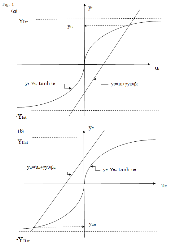
Equations (11) and (12). (a) By introducing a new variable

uI defined by

$$ u _ {I} = \beta_ {I} y _ {I} - \gamma y _ {I I} $$

, Equation (11) is rewritten

into yI = YIst tanh uI. The values of yI are plotted against uI

values according to these first and second equations under

a constant value of yII. The value of yIst satisfying Equation

(11) is determined as the ordinate of the crossing point

of the straight line expressed by the first equation with

the curve expressed by the second equation, as shown

by a broken arrow. The yIst thus determined becomes a

positive value, when the value of yII in the first equation is

chosen to be negative. (b) By introducing a new variable

uII defined by

$$ n _ {i l} = \beta_ {i l} y _ {i l} - \gamma y _ {l} $$

, Equation (12) is rewritten

into yII = YIIst tanh uII. The values of yII are plotted against uII

values according to these third and fourth equations. The

value of yIIst satisfying Equation (12) is determined as the

ordinate of the crossing point of the straight line expressed

by the third equation with the curve expressed by the

fourth equation, as shown by a broken arrow. The yIIst thus

determined is a negative value when the value of yI in the

third equation is taken to be positive. This is consistent

with the result in (a).

Within the framework of the above result, the region $I$ is further divided into the region $I-I$ (leaves) and region $I-II$ (stem), although the region $I-I$ is strictly divided in many sub-regions in most plants. Then, we further consider the master equation of the probability $P(N_{i-1,i+}, N_{i-1,i+}, N_{i-1,i+}, N_{i-1,i+}, N_{i-1,i+}, N_{i-1,i+}, N_{i-1,i+}, N_{i-1,i+}, N_{i-1,i+}, N_{i-1,i+}, N_{i-1,i+}, N_{i-1,i+}, N_{i-1,i+}, N_{i-1,i+}, N_{i-1,i+}, N_{i-1,i+}, N_{i-1,i+}, N_{i-1,i+}, N_{i-1,i+}, N_{i-1,i+}, N_{i-1,i+}, N_{i-1,i+}, N_{i-1,i+}, N_{i-1,i+}, N_{i-1,i+}, N_{i-1,i+}, N_{i-1,i+}, N_{i-1,i+}, N_{i-1,i+}, N_{i-1,i+}, N_{i-1,i+}, N_{i-1,i+}, N_{i-1,i+}, N_{i-1,i+}, N_{i-1,i+}, N_{i-1,i+}, N_{i-1,i+}, N_{i-1,i+}, N_{i-1,i+}, N_{i-1,i+}, N_{i-1,i+}, N_{i-1,i+}, N_{i-1,i+}, N_{i-1,i+}, N_{i-1,i+}, N_{i-1,i+}, N_{i-1,i+}, N_{i-1,i+}, N_{i-1,i+}, N_{i-1,i+}, N_{i-1,i+}, N_{i-1,i+}, N_{i-1,i+}, N_{i-1,i+}, N_{i-1,i+}, N_{i-1,i+}, N_{i-1,i+}, N_{i-1,i+}, N_{i-1,i+}, N_{i-1,i+}, N_{i-1,i+}, N_{i-1,i+}, N_{i-1,i+}, N_{i-1,i+}, N_{i-1,i+}, N_{i-1,i+}, N_{i-1,i+}, N_{i-1,i+}, N_{i-1,i+}, N_{i-1,i+}, N_{i-1,i+}, N_{i-1,i+}, N_{i-1,i+}, N_{i-1,i+}, N_{i-1,i+}, N_{i-1,i+}, N_{i-1,i+}, N_{i-1,i+}, N_{i-1,i+}, N_{i-1,i+}, N_{i-1,i+}, N_{i-1,i+}, N_{i-1,i+}, N_{i-1,i+}, N_{i-1,i+}, N_{i-1,i+}, N_{i-1,i+}, N_{i-1,i+}, N_{i-1,i+}, N_{i-1,i+}, N_{i-1,i+}, N_{i-1,i+}, N_{i-1,i+}, N_{i-1,i+}, N_{i-1,i+}, N_{i-1,i+}, N_{i-1,i+}, N_{i-1,i+}, N_{i-1,i+}, N_{i-1,i+}, N_{i-1,i+}, N_{i-1,i+}, N_{i-1,i+}, N_{i-1,i+}, N_{i-1,i+}, N_{i-1,i+}, N_{i-1,i+}, N_{i-1,i+}, N_{i-1,i+}, N_{i-1,i+}, N_{i-1,i+}, N_{i-1,i+}, N_{i-1,i+}, N_{i-1,i+}, N_{i-1,i+}, N_{i-1,i+}, N_{i-1,i+}, N_{i-1,i+}, N_{i-1,i+}, N_{i-1,i+}, N_{i-1,i+}, N_{i-1,i+}, N_{i-1,i+}, N_{i-1,i+}, N_{i-1,i+}, N_{i-1,i+}, N_{i-1,i+}, N_{i-1,i+}, N_{i-1,i+}, N_{i-1,i+}, N_{i-1,i+}, N_{i-1,i+}, N_{i-1,i+}, N_{i-1,i+}, N_{i-1,i+}, N_{i-1,i+}, N_{i-1,i+}, N_{i-1,i+}, N_{i-1,i+}, N_{i-1,i+}, N_{i-1,i+}, N_{i-1,i+}, N_{i-1,i+}, N_{i-1,i+}, N_{i-1,i+}, N_{i-1,i+}, N_{i-1,i+}, N_{i-1,i+}, N_{i-1,i+}, N_{i-1,i+}, N_{i-1,i+}, N_{i-1,i+}, N_{i-1,i+}, N_{i-1,i+}, N_{i-1,i+}, N_{i-1,i+}, N_{i-1,i+}, N_{i-1,i+}, N_{i-1,i+}, N_{i-1,i+}, N_{i-1,i+}, N_{i-1,i+}, N_{i-1,i+}, N_{i-1,i+}, N_{i-1,i+}, N_{i-1,i+}, N_{i-1,i+}, N_{i-1,i+}, N_{i-1,i+}, N_{i-1,i+}, N_{i-1,i+}, N_{i-1,i+}, N_{i-1,i+}, N_{i-1,i+}, N_{i-1,i+}, N_{i-1,i+}, N_{i-1,i+}, N_{i-1,i+}, N_{i-1,i+}, N_{i-1,i+}, N_{i-1,i+}, N_{i-1,i+}, N_{i-1,i+}, N_{i-1,i+}, N_{i-1,i+}, N_{i-1,i+}, N_{i-1,i+}, N_{i-1,i+}, N_{i-1,i+}, N_{i-1,i+}, N_{i-1,i+}, N_{i-1,i+}, N_{i-1,i+}, N_{i-1,i+}, N_{i-1,i+}, N_{i-1,i+}, N_{i-1,i+}, N_{i-1,i+}, N_{i-1,i+}, N_{i-1,i+}, N_{i-1,i+}, N_{i-1,i+}, N_{i-1,i+}, N_{i-1,i+}, N_{i-1,i+}, N_{i-1,i+}, N_{i-1,i+}, N_{i-1,i+}, N_{i-1,i+}, N_{i-1,i+}, N_{i-1,i+}, N_{i-1,i+}, N_{i-1,i+}, N_{i-1,i+}, N_{i-1,i+}, N_{i-1,i+}, N_{i-1,i+}, N_{i-1,i+}, N_{i-1,i+}, N_{i-1,i+}, N_{i-1,i+}, N_{i-1,i+}, N_{i-1,i+}, N_{i-1,i+}, N_{i-1,i+}, N_{i-1,i+}, N_{i-1,i+}, N_{i-1,i+}, N_{i-1,i+}, N_{i-1,i+}, N_{i-1,i+}, N_{i-1,i+}, N_{i-1,i+}, N_{i-1,i+}, N_{i-1,i+}, N_{i-1,i+}, N_{i-1,i+}, N_{i-1,i+}, N_{i-1,i+}, N_{i-1,i+}, N_{i-1,i+}, N_{i-1,i+}, N_{i-1,i+}, N_{i-1,i+}, N_{i-1,i+}, N_{i-1,i+}, N_{i-1,i+}, N_{i-1,i+}, N_{i-1,i+}, N_{i-1,i+}, N_{i-1,i+}, N_{i-1,i+}, N_{i-1,i+}, N_{i-1,i+}, N_{i-1,i+}, N_{i-1,i+}, N_{i-1,i+}, N_{i-1,i+}, N_{i-1,i+}, N_{i-1,i+}, N_{i-1,i+}, N_{i-1,i+}, N_{i-1,i+}, N_{i-1,i+}, N_{i-1,i+}, N_{i-1,i+}, N_{i-1,i+}, N_{i-1,i+}, N_{i-1,i+}, N_{i-1,i+}, N_{i-1,i+}, N_{i-1,i+}, N_{i-1,i+}, N_{i-1,i+}, N_{i-1,i+}, N_{i-1,i+}, N_{i-1,i+}, N_{i-1,i+}, N_{i-1,i+}, N_{i-1,i+}, N_{i-1,i+}, N_{i-1,i+}, N_{i-1,i+}, N_{i-1,i+}, N_{i-1,i+}, N_{i-1,i+}, N_{i-1,i+}, N_{i-1,i+}, N_{i-1,i+}, N_{i-1,i+}, N_{i-1,i+}, N_{i-1,i+}, N_{i-1,i+}, N_{i-1,i+}, N_{i-1,i+}, N_{i-1,i+}, N_{i-1,i+}, N_{i-1,i+}, N

Click to enlarge

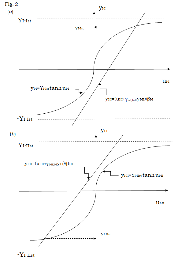
Figure 2: Estimation of yI-I and yI-II values satisfying Equations (25) and (26). (a) Using the new variable uI-I defined by uI-I = βI-IyI-I - γI-I,I-IIyI-II, Equation (25) is rewritten into yI-I = YI-Ist tanh uI-I. The values of yI-I are plotted against uI-I values according to these fifth and sixth equations. The value of yI-Ist satisfying Equation (25) is determined as the ordinate of the crossing point of the straight line expressed by the fifth equation with the curve expressed by the sixth equation, as shown by a broken arrow. The yI-Ist thus determined becomes a positive value, if the value of yI-II in the fifth equation is chosen to be negative. (b) Using the new variable uI-II defined by uI-II = βI-II yI-II - γI-II,I-IyI-I, Equation (26) is rewritten into yI-II = YI-IIst tanh uI-II. The values of yI-II are plotted against uI-II values according to these seventh and eighth equations. The value of yI-IIst satisfying Equation (26) is determined as the ordinate of the crossing point of the straight line expressed by the seventh equation with the curve expressed by the eighth equation, as shown by a broken arrow. The yI-IIst thus determined becomes a negative value when yI-I in the seventh equation is taken to be a positive value. This is consistent with the result in (a). As the strength βI-I and βI-II of the short-range interaction in the respective regions I-I and I-II as well as the strength γI- I,I-II of the long-range interaction between the cells in these regions become greater, yI-Ist and yI-IIst approach to YI-I and - YI-II, respectively, indicating that yI-Ist ≈ - NI-I++/N and yI-IIst ≈ -NI-II+-/N.

The Condition of Cell Differentiation Process to Retain the Meristems

For a simple illustration of this condition, the regions I-I and I-II are treated as the region I in this section. The number No of undifferentiated cells then obeys the following time- change equation.

I II o o o o o d N N e N e N dt

$$ = \lambda_ {o} N _ {o} - e ^ {\alpha I} N _ {o} - e ^ {\alpha I I} N _ {o} \tag {27} $$ The first term on the right hand side of this equation indicates the increase in No with the proliferation rate o λ , while the second and third terms indicate the decrease in No due to the transition to the differentiation mode in the regions I and II with the probabilities eαI and eαII, respectively. In accordance with the above change in the number of undifferentiated cells, the numbers NI+ and NII- of differentiated cells change with time, respectively, by the following equations.

I I I o I d N e N e N dt

$$ I _ {I +} = e ^ {\alpha I} N _ {o} - e ^ {- \alpha I} N _ {I +} \tag {28} $$

II II II o II d N e N e N dt

$$ _ {I I -} = e ^ {\alpha I I} N _ {o} - e ^ {- \alpha I I} N _ {I I -} \tag {29} $$ The second terms on the right hand sides of Equations (28) and (29) indicate the reverse transitions from the differentiated cells to the self-reproducible mode with the probabilities e-αI and e-αII, respectively. The self-reproducible cells returned from these differentiated cells are considered to be transiently marked with the signals characteristic to the respective types of differentiated cells [16], and their numbers NI+o and NII-o increase with time according to the following equations, respectively.

I I o I d N e N dt

$$ I _ {l + o} = e ^ {- \alpha I} N _ {l +} \tag {30} $$

II II o II d N e N dt

$$ _ {I I - o} = e ^ {- \alpha I I} N _ {I I -} \tag {31} $$

If the value of (

$$ \lambda \left(= \lambda_ {o} - e ^ {a l} - e ^ {a l l}\right) $$

is assumed to be time-

independent for simplicity, Equation (27) gives the following

time-dependency of the number No(t) of undifferentiated

cells.

( )

( )exp{ (

$$ N _ {o} (t) = N _ {o} \left(t _ {o}\right) \exp \left\{\lambda \left(t - t _ {o}\right) \right\} \tag {32} $$

In the meantime, the integration of Equation (28) with

respect to time t gives the following time dependence of

NI+(t).

t I I I I o o o I o t N t e t t e N e t d N t α α α τ τ τ − − + + = − − − + ∫

0 ( ) exp{ ( )}[ ( )exp{ ( )} ( )]

(33)

By inserting the expression (32) of $N_o(t)$ into $N_o(\tau)$ on the right hand side of Equation (33), the time-dependency of $N_i(t)$ is reduced to the following form when $t$ is sufficiently larger than $t_o$.

$$N_{i+0}(t) = \frac{e^{aI}}{\lambda + e^{-aI}} N_o(t_o) \exp \left\{ \lambda(t - t_o) \right\}$$

Thus, the following time dependence of $N_{i+0}(t)$ is obtained from Equation (30) when $\lambda \neq 0$.

$$N_{i+0}(t) = \frac{1}{\lambda(\lambda + e^{-aI})} N_o(t_o) \exp \left\{ \lambda(t - t_o) \right\}$$

In the same way, Equations (29) and (31) give the following time-dependence of $N_{i+0}(t)$.

$$N_{i+0}(t) = \frac{1}{\lambda(\lambda + e^{-aI})} N_o(t_o) \exp \left\{ \lambda(t - t_o) \right\}$$

Equations (35) and (36) indicate that $N_o(t) > N_{i+0}(t)$, as long as $\lambda > 1$. This explains the presence of a considerable amount of undifferentiated cells even after the cell differentiation advances to elongate root, stem and leaves. Such undifferentiated cells distribute on the surface of stem and root as well as at their tips called the growth points even in the adult form of the higher plant. In the perennial tree, $\lambda_\theta$ becomes smaller in the winter, but the transition probabilities $e^{aI}$ and $e^{II}$ also become smaller, retaining the relation $\lambda > 1$ in this season.

This is a contrast to the higher animal, where $\lambda$ is nearly equal to zero, or proliferated cells are immediately changed to differentiation mode, and the $N_{i+0}(t)$ and $N_{i+0}(t)$ become larger than $N_o(t)$, forming the "stem cells" for the next stage of cell differentiation in the development [16].

**Cell Differentiation to Form Flowers**

The genetic studies have identified that the light absorbed by the phytochrome initiates the flowering and the homeotic selector genes specify the parts of a flower [23, 24, 25]. However, the seasons of flowering are considerably different between species even in the same district, probably due to the species-specific regulation and control of the following fundamental process. When the biological activity [26] is raised over a threshold by the photosynthesis, it stimulates the proliferation of undifferentiated cells and leads them to express the flower-specific genes under the interaction with the cells forming root, stem and leaves. This process of flowering will be mathematically formulated below.

Under the plausible situation that the formation of flowers does not directly influence the differentiation of first three types of cells described in the third section, the term of $(1 - Y_{i+1} - Y_{i+I} - Y_{iII})$ in Equations (15) and (16) is replaced by $(1 - Y_{i+1} - Y_{i+I} - Y_{iII})$ and the time-change equations of $Y_{iIII}$ and $y_{iIII}$ concerning the fractions of cells in the new region $I-III$ are added. The new variables $Y_{iIII}$ and $y_{iIII}$ are defined by the numbers $N_{iIII++}, N_{iIII++}, N_{iIII++},$ and $N_{iIII++}$ of different types of cells in the region $I-III$.

$$Y_{I-III} = \frac{N_{I-III++} + N_{I-III++} + N_{I-III++} + N_{I-III++}}{N}$$

$$y_{I-III} = \frac{-N_{I-III++} - N_{I-III++} + N_{I-III++} + N_{I-III++}}{N}$$

Each type of cells in the region $I-III$ is characterized by three subscripts; the first and second subscripts are the same as those of the main cells in the regions $I-I$ (leaves) and $I-II$ (stem), interacting with the main cells in the region $II$ (root), and the third subscript – or + – is used for the long-range interaction with the state of main cells in the regions $I-I$ and $I-II$. Accordingly, the cells in the regions $I-I$ and $I-II$ are further characterized by the third subscript +, i.e., the number $N_{i++}$ of +-type of cells and the number $N_{i++}$ of +-type of cells in the third section are modified to $N_{i++}$ and $N_{i++}$ respectively, to indicate the interaction with the cells in the region $I-III$. The total number $N$ of cells is also redefined to $N = N_{i++} + N_{i++}$ and $y_{iIII}$ then obey the following time-change equations, respectively.

$$\frac{d}{dt} Y_{I-III} = \{-Y_{I-III} e^{-aI-III} + 2(1 - Y_{I-1} - Y_{I-II} - Y_{I-III}) e^{aI-III}\}$$

$$\cosh(\beta_{I-III} y_{I-III} - \gamma_{I-III;I-1} y_{I-1} + \gamma_{I-III;I-1} y_{I-II})$$

$$\frac{d}{dt} y_{I-III} = 4Y_{I-III} \sinh(\beta_{I-III} y_{I-III} - \gamma_{I-III;I-1} y_{I-1} + \gamma_{I-III;I-1} y_{I-II})$$

$$-4y_{I-III} \cosh(\beta_{I-III} y_{I-III} - \gamma_{I-III;I-1} y_{I-1} + \gamma_{I-III;I-1} y_{I-II})$$

Here, $\gamma_{I-III;I-1}$ and $\gamma_{I-III;I-1}$ are the strength of the long-range interaction of the cells in the region $I-III$ with the cells in the region $I-II$, respectively, and $\beta_{I-III}$ is the strength of the short-range interaction between the cells in the region $I-III$. The transition probability from the proliferation mode to the differentiation mode in the region $I-III$ is denoted by $e^{aI-III}$ and the probability of reverse transition is denoted by $e^{aI-III}$. Equation (39), together with Equations (15) and (16) modified to replace (1 - YI-I - YI-II - YII) by (1 - YI-I - YI-II - YI-III - YII), indicates that YI-III is directed to the following stationary value YI-IIIst. 2 I III

2 2 2 2 2 1 2 2 2 2

α − I IIIst I I I II I III II e Y e e e e

$$ I _ {I - I I I s t} = \frac {2 e ^ {2 \alpha I - I I I}}{1 + 2 e ^ {2 \alpha I - I} + 2 e ^ {2 \alpha I - I I} + 2 e ^ {2 \alpha I - I I I} + 2 e ^ {2 \alpha I I}} \tag {41} $$ α α α α Equation (40) indicates that yI-III is directed to the stationary value satisfying the following equation.

$$ Y _ {I - I I I} = Y _ {I - I I I s t} \tanh \left(\beta_ {I - I I I} y _ {I - I I I} - \gamma_ {I - I I I, I - I} y _ {I - I} + \gamma_ {I - I I i, I - I I} y _ {I - I I}\right) $$ (42) When the values of yI-Ist and yI-IIst estimated in the preceding section are used for yI-I and yI-II in Equation (42), the value of yI-IIIst can be estimated to be nearly equal to - (NI-III++- + NI-III+-- )/N, as shown in Figure 3.

Click to enlarge

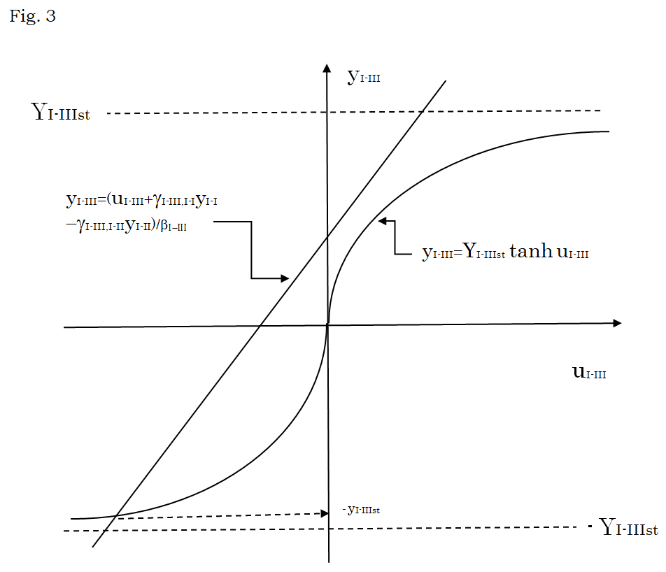
Figure 3: Estimation of yI-III value satisfying Equation (42). By introducing the new variable uI-III defined by uI-III =β I-IIIyI- III - γI-III,I-IyI-I + γI-III,I-IIyI-II, Equation (42) is rewritten into yI-III = YI-III tanh uI-III. The values of yI-III are plotted against the values of uI-III according to these two equations. When yI-I and yI-II are set to be the positive value and the negative value, respectively, that are estimated for yI-Ist and yI-IIst in Figure 2, the value of yI-IIIst is determined to be negative as the ordinate of the crossing point of the straight line with the curve described by above two equations, as shown by a broken arrow. As the strength βI-III of the short-range interaction and the strength γI-III,I-I and γI-III,I-II of the long- range interaction are greater, yI-IIIst becomes nearly equal to - YI-III, indicating that ( ) / I IIIst I III I III y N N N − − ++− − +−− − + . This means that the new region I-III mainly consists of ++- and +-- types of cells, while regions I-I consists of +++ type of cells and the region I-II consists of +-+ type of cells.

Here, NI-III++- and NI-III+ - - correspond to the numbers of cells constituting floral leaf and floral stem, respectively, and their ratio can be also determined by considering the long-range interaction between NI-III++- and NI-III+-- as well as the short- range interaction within each type of cells. Even in some species of deciduous trees, the flower buds are formed before leaf fall and the flowering somewhat precedes the leafing in the spring of next year, but the latter soon grows to supply the former with the nutrient. In this way, the investigation of flowering from the aspect of cell differentiation is necessary to the physiological study of flowering, in addition to the trigger by the phytochrome accepting light.

Although the mathematical description of the further differentiation of the cells in yI-III type to form the pistil, stamen and seed is reserved for the next paper, the regulation and control of this process forming seeds gives a measure for the separation of annual plants from the perennial plants. First of all, the appearance of the region I-III leading to flowering decreases the apparent increase rate λ of undifferentiated cells in Equations (32) ~ (36) to $$ \lambda_ {f} = \lambda_ {o} - e ^ {a l} - e ^ {a l l} - e ^ {a l - l l}. $$

. Second, the plant endows the

fertilized eggs produced by pollination with a considerable

amount of materials and energy to form seeds. This lowers

the proliferation rate

o

λ itself of undifferentiated cells. In

the annual plant,

f

λ becomes zero or a negative value, and

the numbers NI-I+++, NI-II+-+ and NII- of cells are so decreased not

to compensate for the dead cells in leaves, stem and root.

The perennial plant, on the contrary, reserves the materials

and energy for the budding in the next season by producing

a less number of smaller seeds in comparison with the size

of the plant body.

Conclusions and Discussion

In the higher plant, the proliferation rate of undifferentiated cells is faster than the transition rate to the differentiated cells, and the self-reproducible undifferentiated cells are retained at the peripheral parts even in the adult form. Thus, the ratios of the numbers of cells forming root, stem and leaves, respectively, are directed to be determined in a straightforward way by the transition probability of a cell from the self-reproducible mode to the differentiation mode and by both the long-range interaction between the distinctive types of cells and the short-range interaction between the same type of cells, even if the ligand- receptor and intracellular phosphorylation signal underlying the long-range and short-range interactions are essentially common to both the higher plant and the higher animal.

This style of cell differentiation process explains the following high ability of regeneration in the higher plants by considering that the partial removal of differentiated cells stimulates the proliferation of undifferentiated cells to recover the ratio of root, stem and leaves, utilizing the energy and materials accumulated by the photosynthesis. Many species of grasses regenerate blades from the left root even if the blades are pinched off. Most of perennial trees show the side growth of shoots when the tips of branches are pinched off and some species of them further generate roots from a separated branch when it is put into the soil. Some of angiosperms have further evolved to deciduous trees extending this property for the survival against cold winter. It is a future problem to ascertain the compatibility of the molecular mechanism underlying the cell differentiation with the plant hormones. In contrast to the animals where hormone production is restricted to specialized glands, each plant cell is capable of producing hormones. The well-known example is the auxin which alone promotes root formation, in conjunction with gibberellin it promotes stem elongation, with cytokinin it suppresses lateral shoot outgrowth, and with ethylene it stimulates lateral growth [27]. In addition, it is now reported that plant hormones control many aspects of growth and development, from embryogenesis [28], pathogen defense [29, 30], stress tolerance [31, 32], and through the reproductive development [33].

Moreover, not a few groups of higher plants perform the vegetative reproduction or clonal growth as well as the gamete reproduction, utilizing the self-reproducible undifferentiated cells in the developed subterranean stem. The well-known examples of vegetative reproduction from the subterranean stem are seen in the white or Irish potato belonging to Salanaceae and in the sweat potato belonging to Convolvulaceae. The bamboo shows the clonal growth somewhat different from the vegetative reproduction in potatoes. It puts forth buds called the bamboo shoots in the spring of every year and each shoot grows to almost a definite size of root, stem and leaves within one year. The bamboo forest thus constructed under a connected subterranean stem suddenly blooms and dies after more than one hundred years. In these plants, it is necessary to consider the division of the region II into the region II-I (root) and the region II-II (subterranean stem) and to identify the signal transmission that rouses the vegetative reproduction or clonal growth from the undifferentiated cells in the subterranean stem. According to the study of evolution [34], the land plants have started from Bryophyta, from some of which Pterophyta have then appeared by acquiring vascular bundle, and finally Gymnospermae and Angiospermae have appeared. This means that the cell differentiation in land plants first occurs to form root, leaf and simple spores, and the flowering becomes possible after the formation of stem by acquiring the vascular bundles. The clonal growth from subterranean stem is also observed on Sphenopsida, which seems to have appeared at almost the same ancient time as Pterophyta. Thus, the clonal growth is also another strategy than the gamete reproduction for survival from the early stage of evolution in higher plants, although the vegetative reproduction and clonal growth are inferior to the gamete reproduction in acquiring the combination of new genes.