Diffusion Coefficient Measurements of T1-Enhanced Contrast Agents in Water Using 0.3 T Spin Echo Proton MRI

Agarose Gel Plate for Diffusing CAs and Size of Image Element of MRI

Figure 1 shows a prepared gel plate in a container. The concentration of agarose gel (Wako, Tokyo, Japan) in pure water (18.2 MΩ·cm at 25°C) is 1.0% w/v because water in 1.0% (w/v) agarose gel is similar to free water and because thermal convection, which can disturb the diffusion motion of CAs in water, is restricted by agar gel. The gel plate was positioned horizontally in the container. The width, height, and thickness of the plate were 110.0, 110.0, and 1.0 mm, respectively. The gel plate had eight rectangular grooves oriented in the vertical direction and spaced 6 mm apart. The grooves were 4.0 mm in height, 1.0 mm in width, and 1.0 mm in depth. The x and y axes of the gel plate were oriented in the horizontal and vertical directions, respectively, with the origin of the x axis located at the center of the rectangular grooves. Hence, the left and right edges of the gel plate were at x = -60.0 and +50.0 mm, respectively, and those of the rectangular grooves were at x = -0.5 and +0.5 mm.

Click to enlarge

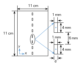
The four CAs prepared were Gd-DTPA (Magnevist, Bier, Switzerland), Gd-HP-DO3A (gadoteridol Prohance, Bracco Eizai, Japan), MnCℓ2 (Tokyo Kasei, Tokyo, Japan), and albumin-(Gd-DTPA) (M.W. 94000) (Contrast Media Lab., San Francisco, CA, USA) [2]. The M.W. increase of 94000 of albumin-(Gd-DTPA) from 66000 of HSA is caused by addition of 30 Gd-DTPAs bound to HSA. Contrast solutions were made by adding pure water to the CAs. Because the concentration of a contrast solution is defined in terms of the concentration of paramagnetic ions, such as Gd$^{3+}$ and Mn$^{2+}$, that of albumin-(Gd-DTPA) is measured by the Gd concentration and not by the albumin concentration. Eight contrast solutions with concentrations of 0.25, 0.50, 0.75, 1.0, 1.5, 1.75, 2.0, and 4.0 mmol/$\ell$ were placed in the eight rectangular grooves at $t = 0$ h, where $t$ is the time. The initial concentrations of the eight contrast solutions were at their peaks at the groove centers.

Imagining was carried out using the AIRIS Vento MRI machine (Hitachi, Tokyo, Japan), operated at 0.3 T. The gel plate was mounted on a birdcage coil tuned for protons, the temperature of which was maintained at 25°C. MR imaging was performed with a T${1}$-weighted spin echo pulse sequence, where $T{1}$ was the spin-lattice relaxation time. The repetition time (TR) and echo time (TE) were 400 and 15 ms, respectively. The slice thickness was 2.0 mm, which was the thickness of the gel plate. The field of view was 180 mm $\times$ 180 mm in the x and y directions, respectively. The frequency and phase axes were the x and y axes, respectively, and the division numbers in those directions were set to $N_x = 256$ and $N_y = 224$, yielding an acquisition matrix of size $256 \times 224$. The number of signal averages (NSA) was set to four. The total scan time $\tau$ required to obtain one MRI is derived as follows:

$$\tau = \text{TR} \times N_y \times \text{NSA.}$$

(1)

For the above values, Equation 1 yields $\tau = 6$ min (358.4 s). Because the diffusion motion of the CAs was measured in the x direction, the image element size $\Delta$ in the x direction had to be determined precisely. We calculated it to be 703.1 $\mu$m [(180/256) mm]. Because the display matrix size increased up to 512 $\times$ 512, which is approximately twice the size of the acquisition matrix, $\Delta$ in the output display was reduced to 351.6 $\mu$m [(180/512) mm].

Linearity between proton MRI signal intensity and CA concentration

The paramagnetic ions Mn$^{2+}$ and Gd$^{2+}$ shorten the spin-lattice relaxation time $T_{1}$ and spin-spin relaxation time $T_{2}$ of the protons around them. These times are related to the paramagnetic ion concentration [C] through:

$$\frac{1}{T_1} = \frac{1}{T_{1,0}} + R_1[C], \quad \frac{1}{T_2} = \frac{1}{T_{2,0}} + R_2[C] \quad (R_1 < R_2)$$

(2)

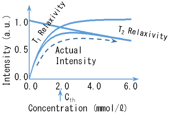
where $T_{1,0}$ and $T_{2,0}$ are the $T_{1}$ and $T_{2}$ of pure water, respectively, and $T_{1,0} = T_{2,0} = 3.6$ s. The proportional coefficients $R_1$ and $R_2$ are called $T_{1}$ and $T_{2}$ relaxivities, respectively, and have units of $1/((\text{mmol}/\ell) \cdot \text{s})$. When MR imaging is performed with a $T_{1}$-weighted pulse sequence, the proton signal intensity (SI) is expressed as follows [1]:

$$\text{SI} \propto \left(1 - \exp \left(-\frac{\text{TR}}{T_1}\right)\right) \exp \left(-\frac{\text{TE}}{T_2}\right) \quad \text{TR} > \text{TE}$$

(3)

where TE $<< T_2$. The dependence of the SI on C, assuming that $R_1 = 3.4$ and $R_2 = 4.0$ in Equation 2 [1] and that TR = 0.4 and TE = 0.015 s in Equation 3, is plotted in Figure 2 [15]. When [C] is lower than the saturation concentration $[C]{th}$ of 1.0 mmol/$\ell$, TR $<< T_1$ and TE $<< T_2$ hold because $T{1}$ and $T_{2}$ are greater than 1 s. Therefore, for $C \leq C_{th}$, the approximations $\exp(-\text{TR}/T_1) \equiv 1 - \text{TR}/T_1$ and $\exp(-\text{TE}/T_2) \equiv 1$ hold and Equation 3 becomes

$$\text{SI} \propto \text{TR} \cdot R_1 \cdot [C]$$

(4)

The linearity between SI and C described by Equation 4 is desirable for observing the diffusion motion of the CA in water using MRI. The maximum paramagnetic concentration that satisfies Equation 4 should be checked for each set of experimental conditions. There is nearly proportionality between R1 and R2 for each CA. The R1 and R2 of low-molecular- weight CAs such as Gd-DTPA are lower than those of high-molecular-weight CAs such as albumin-(Gd-DTPA) [1, 2, 3, 14].

Click to enlarge

Quasi-Gaussian Concentration Profile Produced by Brownian Motion

A molecule of a CA is considered to be a sphere of radius a and mass M, and we perform a translational motion in the x direction in a Newtonian fluid of liquid water. The diffusion of the CA in water is caused by random-walk translational motion caused by random collisions referred to as Brownian motion. The diffusion coefficient D and diameter 2a of the molecule are related by the Einstein’s formula as follows [16]:

(5) where kB, T, and η are the Boltzmann constant (1.38 × 10-

$$ \mathrm {D} = \frac {\mathrm {k} _ {\mathrm {B}} \mathrm {T}}{6 \pi \mathrm {a n}} $$ a 6 η π

23 J/K), the temperature in degrees Kelvin, and the water viscosity at 25°C (0.890 × 10-3 Pa·s), respectively. Although the molecular net charge of a CA such as Gd- DTPA modifies the diffusion coefficient in water, the effect is small at the clinical dose concentration of 0.5 mmol/ℓ [12, 13].

The concentration profile C(x,t) of the contrast solution depends on x and t because the solution expands out of the groove with time, due to Brownian motion. Because the rectangular groove is thin in the x direction (1 mm), an analysis of the slab geometry in the x direction is possible. When the width d of the groove is assumed to be infinitely narrow, the concentration profile of the CA diffusing in the x direction is described by a Gaussian profile [17]: (6)    $$ = \frac {1}{\sqrt {4 \pi \mathrm {D t}}} \exp \left(- \frac {x ^ {2}}{4 D t}\right) $$

2

1 t x, C

( )   π The evolution of the Gaussian profile with time is shown in Figure 3(a1). The initial concentration profile just after the addition of the contrast solution at t = 0 h is expressed as follows:

$$ \mathrm {C} \left(\left| \mathrm {x} \right| \leq \frac {\mathrm {d}}{2}\right) = 1. 0, \quad \mathrm {C} \left(\left| \mathrm {x} \right| > \frac {\mathrm {d}}{2}\right) = 0. 0 $$ (7) To incorporate the finite groove width d in Equation 6, the relaxation time trel is introduced as shown below:

$$ \mathrm {d} = 2 \sqrt {\mathrm {D} t _ {r e l}} $$

(8) When t = trel, Equation 6 yields C(x = ±d/2) = e-1/4× C(x = 0)≃ 0.78 × C(x = 0) and C(x = ±d)= e-1 × C(x = 0)≃ 0.37 × C(x = 0), which is similar to the initial profile described by Equation 7. Thus, by incorporating Equation 8, Equation 6 is transformed into a quasi-Gaussian profile, expressed as follows:

    = −    

2

1 C x, t + t exp 4 t + t 4 D t + t x D π

( ) (9) ( ) ( )

rel rel rel

The half-width position $x_{\text{half,t}}$ satisfying $\exp(-x_{\text{half,t}}^2/4D (t + t_{\text{rel}})) = 1/2$ in Equation 9 displaces over time and is written as

$$x_{\text{half,t}} = 1.39 \sqrt{D(t + t_{\text{rel}})}$$ (10)

where $1.39$ is $2(\log_2 2)^{1/2}$. When the diffusion coefficients $D$ of MnC$\ell_2$, Gd-DTPA, and albumin-(Gd-DTPA) are assumed to be $1.3 \times 10^{-9}$, $0.4 \times 10^{-9}$, and $0.06 \times 10^{-9} \text{ m}^2/\text{s}$, respectively, the $t_{\text{rel}}$ values for the three CAs are 46 s, 2 min 30 s, and 16 min 40 s, respectively. The half-width ratios among MnC$\ell_2$, Gd-DTPA, and albumin-(Gd-DTPA) are approximately 9:5:2 after $t = t_{\text{rel}}$. These ratios were calculated from $1.3^{1/2}; 0.4^{1/2}; 0.06^{1/2}$ in Equation 10 [14].

Exact Numerical Simulation of Concentration Profile Determined by Diffusion Coefficient

Because the Gaussian profile in Equation 6 assumes that all molecules are located in an infinitely narrow groove at $x = 0$ before the start of diffusion (for $t \leq 0$) and that the concentration $C(x,t)$ becomes infinity at $x = 0$ and $t = 0$, numerical simulation is required to determine the exact concentration profile of the CA diffusing from a 1-mm-wide groove. The displacement $x$ and time $t$ are divided into a series of thin shells of thickness $\Delta x$ and $\Delta t$, respectively and are denoted by numbers $k = 1, \ldots, = x/\Delta x$ and $n = 1, \ldots, t/\Delta t$, respectively. The shells are denoted with subscripts from 1 to max, where $x_1 = -60.0 \text{ mm}$ and $x_{\text{max}} = 50.0 \text{ mm}$ correspond to the left and right edges of the shell, respectively.

The concentrations of the shells are denoted $C_1$ to $C_{\text{max}}$. The number and concentration of each shell are defined at its center. Diffusion motion is numerically calculated from the concentration gradient between adjacent shells. Because a molecule exhibiting Brownian motion reflects at the left and right edges of the gel plate, two outer shells $C_0$ and $C_{\text{max}+1}$ should be located at the left of $C_1$ and right of $C_{\text{max}}$, respectively, for the reflection boundary conditions. The initial peak concentrations added to the eight grooves were normalized to one because the diffusion coefficient is not affected by the concentration at levels close to the clinical dosage of 0.5 mmol/$\ell$ [12, 13]. The diffusion starts from the initial concentration profile of Equation 7 at $t = 0$. After $t = 0$, the reflection boundary conditions are set as $C_1 = C_0$ at $x = x_1$ and $C_{\text{max}} = C_{\text{max}+1}$ at $x = x_{\text{max}}$.

The concentration in the $k^{\text{th}}$ shell ($k = 1, \ldots, \text{max}$) changes as a result of the transport between the adjacent shells at each time step $\Delta t$, which is proportional to the product of the concentration gradient and the diffusion coefficient, according to the following difference scheme:

$$\Delta x \frac{C_{\text{k}}^{n+1} - C_{\text{k}}^n}{\Delta t + t_{\text{rel}}} = D \left[ \frac{C_{\text{k}+1}^n - C_{\text{k}}^n}{\Delta x} + \frac{C_{\text{k}+1}^n - C_{\text{k}}^n}{\Delta x} \right]$$ (11)

Here, the superscript $n$ of $C_k$ denotes time step $\Delta t$. During the numerical simulation, $C_{\text{k}+1}^n$ shifts to $C_{\text{k}}^n$ at the next time step. The scheme of Equation 11 is called an explicit scheme, where $\Delta t$ should satisfy $\Delta t < (\Delta x)^2/(2D)$ to provide stable numerical simulations[18, 19]. To perform numerical simulations that yield an error less than $1\%, \Delta x$ should be smaller than $10.0 \mu\text{m}$, which is one hundredth of the groove width.

The analytical profile diffusing from an infinitely narrow groove, derived from the Gaussian profile in Equation 6, and the numerical profile diffusing from a 1-mm-wide groove, derived from numerical simulation using Equation 11, are shown for $t = 0, 24, 60$, and 120 min in Figures 3(a1) and (a2), respectively, where the pixel size is $\Delta = 351.6 \mu\text{m}$ and the diffusion coefficient $D$ is set to be $0.06 \times 10^{-9} \text{ m}^2/\text{s}$. Those analytical and numerical profiles are symmetric with respect to $x = 0$ and exhibit similar linear tails forming isosceles triangles in the $x^2$-log$_{10}$C plane (denoted analytical (AT) and numerical tails (NT) and shown on the left and right of Figure 3(b1), respectively), from the peak concentration to the position at which the concentration is one hundredth of the peak concentration—as most of the signal peaks. Because the quasi-Gaussian profile in Equation 9, including the finite groove width $d$, is also an analytical profile, the AT calculated from Equation 9 is denoted by AT'. The widths of the AT, AT', and NT are determined between the linear tail ends spreading with time. The AT and AT' are typical properties of the Gaussian profile. The width of the NT is slightly greater than that of the AT because of the groove width $d$. The difference |NT–AT| is shown on the right in Figure 3(b1). Time-shift arrangements of AT and NT are compared on the left and right sides of Figure 3(b2), respectively. The different times corresponding to the three diffusion coefficients D = 0.06 × 10-9, 0.4 × 10-9, and 1.3 × 10-9 m2/s are indicated in the vertical axis in Figure 3(b2). Because the diffusion coefficient D is proportional to x2 rather than x, as shown in Equations (6) and (9), the rates of change of the differences between NT and AT and between NT and AT′ are defined as (NT2 − AT2)/NT2 and (NT2 − AT′2)/NT2, respectively. These rates are highest just after the start of diffusion. Until some point in time, the higher rates are expected to be maintained because of the finite width groove. Because this point in time occurs later when d is larger or D is smaller and because d2/D has units of time, we can measure time in terms of d2/D. This is done in Figure 3(c), which shows that the “Gaussian” (NT2 – AT2)/NT2 and and “quasi-Gaussian” (NT2 – AT′2)/NT2 difference rates decrease with time, and reach below 0.1 after t = 0.12 × d2/D (= 0.48 trel) and 0.36 × d2/D (= 1.44 trel), respectively, where trel = 0.25d2/D in Equation 8 is indicated by the upward arrow in the horizontal axis. Thus, the quasi-Gaussian profile in Equation 9 is a good approximate formula for use in the numerical calculation and is expected to yield the diffusion coefficient of a CA within a 10% error margin after t = 0.48 trel without numerical simulation. The actual times corresponding to 0.48 trel were found to be 1 min 32 s, 5 min, and 33 min 20 s for D = 1.3 × 10-9, 0.4 × 10-9, and 0.06 × 10-9 m2/s, respectively. (The different times corresponding to these three diffusion coefficients are shown in the x axis of Figure 3(c).) The approximate formula for the decrease in the peak concentration Cpeak with time is derived from Equations 8 and 9 and reads:

C

t = C

peak rel (12) t + t =

rel

0 t peak, where Cpeak,t=0 is the peak concentration at t = 0. Figures 3(d1) and (d2) compare the numerically simulated peak concentration Cpeak and approximate peak concentration Cpeak,approx determined from Equation 12, where the time scales of the horizontal axes are similar to that in Figure 3(c). In Figure 3(d1) we see that Cpeak,approx (labeled as “Quasi-Gaussian”) and Cpeak (“Numerical Simulation”) decrease and become closer with time. The evolution of the ratio (Cpeak − Cpeak,approx)/Cpeak over time is shown in Figure 3(d2). Because this ratio reaches a maximum of

0.16 at t = 0.06 × d2/D and remains at 0.12 after t = trel (= 0.25 × d2/D), Equation 12 was found to be a practical formula to estimate the peak concentration without numerical simulation.

Click to enlarge

Click to enlarge

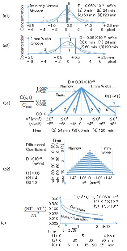
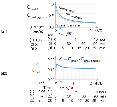
Figure 3: Time evolution of the concentration profiles C(x,t) diffusing from (a1) an infinitely narrow groove and (a2) a 1-mm-wide groove, represented by linear tails in the x2-log10C(x,t) plane in the left and right parts of (b1), respectively. Because the profiles of (a1) and (a2) were derived analytically and numerically, respectively, the linear tails to the left and right in (b1) are denoted an analytical tail (AT) and numerical tail (NT), respectively. The NT (right) is greater than the AT (left) because the groove width is considered in the numerical simulation. (b2) Time-shift arrangement of AT (left) and NT (right), for concentrations greater than 0.1 of the peak concentrationes at each time step. (c) The difference (NT2 − AT2)/AT2 between the NT and AT decreases with time. The AT of the quasi-Gaussian profile is closer to the numerical profile than that of the Gaussian profile. (d1) Time progression of the peak concentrations derived from the numerical simulation Cpeak and quasi-Gaussian profile Cpeak,approx. (d2) Time evolution of the ratio (Cpeak− Cpeak,approx.)/Cpeak,. which is always less than 0.16.

MR Imaging Affected by Diffusion Motion During Scan Time

The half-width position xhalf,t in Equation 10 is illustrated in Figure 3(b1) and displaces with time t. The velocity dxhalf/dt of xhalf,t at the start of MRI (t = tstart) is calculated as follows:

rel x D = 0.7 dt t + t d (13)

half where 0.7 is 1.39/2. The displacement of xhalf,t generated during the MRI scan time τ (from t = tstart to t = tstart + τ) is denoted by ⊿xhalf,t,τ. If ⊿xhalf,t,τ exceeds the size of one image element ⊿ (= 351.6 μm), that is, ⊿xhalf,t,τ/⊿ > 1, the measurements of CA diffusion coefficients obtained using MRI with finite τ include errors. Equation 10 evaluates ⊿xhalf,t,τ exactly as follows [14]:

    + + −      

$$ \mathrm {x} _ {\mathrm {h a l f}, t, \tau} = 1. 3 9 \left(\sqrt {\mathrm {D} \left(\mathrm {t} _ {\mathrm {s t a r t}} + \tau\right) + \frac {d ^ {2}}{4}} - \sqrt {\mathrm {D t} _ {\mathrm {s t a r t}} + \frac {\mathrm {d} ^ {2}}{4}}\right) $$ τ (14) When the diffusion and MRI start simultaneously (tstart = 0), ⊿xhalf,t,τ is derived from Equation 14 by setting tstart = 0 and is denoted by ⊿xhalf,0,τ:

   $$ \square x _ {\mathrm {h a l f}, 0, \tau} = 1. 3 9 \left(\sqrt {\mathrm {D} \tau + \frac {\mathrm {d} ^ {2}}{4}} - \frac {\mathrm {d}}{2}\right) $$

2 (15)   half,0, τ ⊿

Equations 14 and 15 reveal that a lower D, shorter tstart, and shorter τ will yield a lower ⊿xhalf,t,τ/⊿, which is understood from the diffusion velocity in Equation 13. The dependence of ⊿xhalf,0,τ/⊿ in Equation 15 on τ is illustrated in Figure 4(a), where the upper and lower curves correspond to high (D = 1.3 × 10-9 for MnCℓ2) and low (D = 0.4 × 10-9 m2/s for Gd-DTPA) diffusion velocities, respectively. The displacement ⊿xhalf,0,τ exceeds ⊿ (⊿xhalf,0 /⊿ ≧ 1) when τ is longer than 4 and 13 min for the high and low diffusion coefficients, respectively. The time ratio 4:13 is the inverse ratio between the high and low diffusion coefficients as understood from Equation 15. Thus, the MRI performed using a scan time of τ = 6 min in this study permitted observation of the low-velocity diffusion of Gd-DTPA without error (⊿xhalf,0/⊿ ＜ 1) for any choice of tstart ≧ 0 but did not permit observation of the high-velocity diffusion of MnCℓ2 without error as long as tstart = 0. With increasing tstart, ⊿xhalf,t,τ decreases because ∂⊿xhalf,t,τ/∂tstart < 0 in Equation 14. The dependence of ⊿xhalf,t,τ/ ⊿ on tstart for high diffusion velocity (D = 1.3 ×10-9 for MnCℓ2) derived from Equation 14 is shown in Figure 4(b), where the upper and lower curves correspond to longer (τ = 6 min) and shorter (τ = 1.5 min) scan times, respectively. Even when τ = 6 min, the MRI permitted observation of this high-velocity diffusion without error when tstart > 1.5 min, whereas for τ = 1.5 min there was no error for any choice of tstart ≧ 0. Equation 1 indicated that τ is proportional to the NSA and the phase division number Ny. Because of this, the standard τ = 6 min is determined from Ny = 224 and NSA

= 4. It is better to set NSA ≧ 4 for 0.3 T MRI to perform high-resolution MRI. MRI with τ = 1.5 min permits observation of high-velocity diffusion without error when Ny is changed to from 224 to 56 (= 224/4). High-Tesla MRI is useful in tracing high-velocity diffusion because NSA = 1 is sufficient for obtaining high-resolution MR images [14]. If the spatial variation along the phase axis is low, an increase in NSA from 4 to 16 and a decrease in Ny from 224 to 56 will lead to higher-resolution MRI without changing the scan time of τ = 6 min.

Click to enlarge

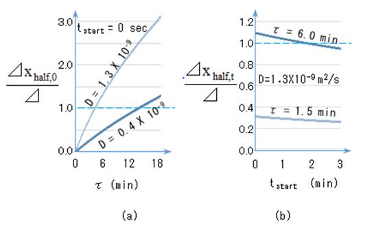
Figure 4: The half-width position of the quasi-Gaussian profile displaces due to diffusion during the MRI scan time τ by ⊿xhalf,0 when the MRI starts, just after the start of diffusion (tstart = 0). The diffusion measurement using MRI contains errors if ⊿xhalf,0 exceeds the size of one image element ⊿ (= 351 μm) during τ. (a) The displacement ⊿xhalf,0 increases with τ and exceeds ⊿ after τ = 4 and 14 min for D = 1.3×10-9 and 0.4×10-9 m2/s, respectively. (b) When the MRI for high- velocity diffusion (D = 1.3 × 10-9 m2/s ) starts after the start of diffusion (at t = tstart), ⊿xhalf,t decreases with increasing tstart. ⊿xhalf,t is always less than ⊿ when τ is set to 1.5 min, whereas for τ = 6.0 min ⊿xhalf,t is greater than ⊿ when the MRI begins between 0 and 1.6 min after the start of the diffusion (tstart = 0–1.6 min).

Linearity between the Signal Peak Amplitude and Peak Concentration in Rectangular Grooves

Four contrast solutions in eight different concentrations were initially added to the eight rectangular grooves on the agar gel plate at 25℃ at time t = 0 h, as shown in Figure 1. MR images for the four contrast solutions of Gd-DTPA, Gd-HP-DO3A, MnCℓ2, and albumin-(Gd-DTPA) at t = 0 h are shown in Figure 5(a0). The eight vertically oriented rectangular grooves were numbered from one to eight (the corresponding numbers Ngrv are shown on the right side in descending order), and the concentrations increased vertically upward. The white region in Figure 5(a) corresponds to a normal proton signal from pure water without a CA. The gray and black regions correspond to the low and high concentrations of the CAs, respectively, because the proton SI increases with the CA concentration (see Equation 4 and Figure 2). Thus, the upper solutions with the highest concentrations exhibit the highest SIs among the eight contrast solutions. The origin of the y axis is indicated by the darkest dot in the upper left of the gel plate, while the origin of the horizontal displacement (x axis) is located at the groove center. MR images of the four gel plates of the four CAs after one hour (t = 1 h) are shown in Figure 5(a1). Bird’s-eye views of the proton SI around the grooves at t = 0 h and 1 h are compared in contour maps shown in Figures 5(b0) and (b1), respectively. The eight grooves produce eight signal peaks with finite distribution diameters and located (as the peak concentrations) at the groove centers (x = 0). The distribution diameters of the eight signal peaks at t = 1 h Figure 5(b1) are greater than the initial ones at t = 0 h Figure 5(b0). The random-walk diffusion motion of the CAs is evident from the expanding high SI regions in the Gaussian profiles around the grooves. Because the widths of the rectangular grooves, measured in the horizontal (x) direction is 1 mm and the size of one image element is 351.6 μm, there are two vertical image lines crossing around the signal peak. By averaging the SIs measured along the two image lines crossing the eight rectangular grooves, the eight signal peaks at t = 0 and t = 1 h (estimated by numerical simulation using Equation (11)) are shown in Figures 5(c0) and (c1), respectively. The horizontal and vertical axes correspond to the proton SI in arbitrary units (a.u.) and Ngrv (y axis), respectively. Background signal levels are evident under the eight signal peaks. If the eight peak concentrations at t = 1 h are estimated using the approximate formula in Equation 12, the error in the numerical simulation results obtained using Equation 11 is within 1%, as discussed in Exact Numerical Simulation of Concentration Profile Determined by Diffusion Coefficient. The initial peak concentrations of the eight rectangular grooves are not proportional to Ngrv. The relation between the eight signal peak amplitudes at t = 0 h and the initial peak concentrations is shown in Figure 5(d0), where the background signals have been eliminated. The SIs and CAs concentration are linearly related at concentrations below the saturation concentration Cth of approximately 2 mmol/ℓ at t = 0 h, as indicated by Equation 4. The rate of increase of SI is described by Equation 3 for concentrations above the saturation concentration (C > Cth). Because, as Equation 9 describes, the eight signal peak amplitudes decrease with time for similar values of (2D(t + trel))-1/2, the ratios among the eight peak concentrations do not change with time. The relation between the eight observed signal peak amplitudes and the numerically simulated peak concentrations at t = 1 h is shown in Figure 5(d1). Because of the decrease in the peak concentration with time, linearity extends to almost all the signal peaks (from Ngrv = 1 to Ngrv = 8) for the Gd- DTPA, Gd-HP-DO3A, and MnCℓ2 CAs and the lower- concentration signal peaks from Ngrv = 5 to Ngrv = 8 for the albumin-(Gd-DTPA) CA at t = 1 h. Because the diffusion coefficient of albumin-(Gd-DTPA) is less than one hundredth of that of Gd-DTPA, the decrease in the peak concentration at t = 1 h is noticeably smaller than for other CAs. Furthermore, the R1 of albumin-(Gd-DTPA) is the greatest among the four CAs, and as a result there is no linearity between the concentration and the SI from Ngrv = 1 to Ngrv = 4 at t = 1 h. Hence, the linearity discussed in Linearity between Proton MRI Signal Intensity and CA Concentration and described by Equation 4 is satisfied at t = 1 h, and thus the diffusion coefficients of the four CAs in water can be determined from the SI profiles. The MRI is not affected by diffusion motion during the scan time of 6 min at t = 1 h, as discussed in MR Imaging Affected by Diffusion Motion During Scan Time.

Diffusion Coefficients of CAs Determined from Proton Signal Intensity Profiles

The eight intensity profiles varying along the horizontal image lines and crossing the eight signal peaks at t = 0 and 1 h are shown in Figures 5(e0) and (e1), respectively, where the proton SI is measured in a.u. and the groove numbers (Ngrv = 1 to 8) are shown at the left. The initial and numerically simulated peak concentrations at t = 0 h and 1 h, respectively, are indicated at the right in Figures 5(e0) and (e1), respectively. Because the peak concentration decreases with time, a bidirectional arrow between Figures 5(e0) and (e1) indicates that the lower peak concentration (Ngrv > 1 ) at t = 0 h is close to the highest peak concentration (Ngrv = 1) at t = 1 h. Because the height of the rectangular groove is 4 mm and the size of one image element is 351.6 μm, there are multiple horizontal image lines crossing around the signal peak. Because diffusion occurs in both the x and y directions, the proton SI decays from the signal peak in both directions. Thus, the five horizontal image lines (x axis) crossing around the signal peak exhibit similar intensities, and other lines outside them exhibit lower intensities. Figure 5(e) consists of the upper and lower parts for all grooves (Ngrv = 1 to 8). Five intensity profiles along the five horizontal image lines are shown in the upper part, and one intensity profile, obtained by averaging the five profiles along the five horizontal image lines, is shown in the lower part. The signal peaks at the center of the intensity profile are located at the groove centers at x = 0. The amplitudes of the signal peaks are normalized to be one at the eight grooves at t = 1 h in Figure 5(e1), where the background noise levels are schematically indicated by short vertical bars with “noise” for Ngrv = 4 and 5 in Gd- DTPA and for N grv = 5 and 6 in MnCℓ2. The SNRs become lower in the lower peak concentration grooves for Gd- DTPA, Gd-HP-DO3A, and MnCℓ2 for N grv ≧ 5. The line indicating the midpoint SI level between the bottom and the peak is plotted for each groove in Figure 5(e1) at t = 1 h. The amplitudes of the signal peaks are not normalized at t = 0 h in Figure 5(e0). Three lines indicating one- quarter, one-half, and three-quarter SI levels are plotted at each groove in Figure 5(e0). Because these three levels are absolutely fixed, we can easily appreciate the increase in the signal peak amplitude with the peak concentration. The initial SI profile at t = 0 h in Figure 5(e0) is not the step-like profile in Equation 7 but a Gaussian-like profile, mainly because MRI with a fundamental image element size of 351.6 μm cannot accurately characterize a 1-mm groove width. The peak and bottom signal intensities are determined as SI = 1.0 and SI = 0.0, respectively, in the intensity profile at t = 1 h (Figure 5(e1)). 15 intensity levels are defined between the peak and bottom, where the intensity step is 0.067. Because each equi-intensity line has two intersections with the intensity profile, the width wd is determined between the two intersection points at each intensity step, and x2 is defined as x2 = (wd/2)2. The intensity profiles at t = 1 h are plotted by 15 experimental dots at the 15 intensity levels in the x2–log10SI plane in Figure 6. Because the SNR is low for Gd-DTPA, Gd-HP- DO3A, and MnCℓ2 for Ngrv = 5 to 8, as shown in Figure 5(e1), experimental dots are shown for Ngrv = 1 to 4 in Figure 6, which illustrates the linearity between the SI and the peak concentration. Because there is no linearity between the SI and the peak concentration of albumin- (Gd-DTPA) for Ngrv = 1 to 4, as shown in Figure 5(e1), experimental dots are shown for Ngrv = 5 to 8 in Figure 6, where the SNR is sufficient. The noise levels relative to the signal peaks at t = 1 h, as shown in Figure 5(e1), are 0.15 (Ngrv = 1), 0.27 (Ngrv = 2), 0.23 (Ngrv = 3), and 0.23 (Ngrv = 4) for Gd-DTPA; 0.15 (Ngrv = 1), 0.36 (Ngrv = 2), 0.42 (Ngrv = 3), and 0.48 (Ngrv = 4) for Gd-HP-DO3A; 0.12 (Ngrv = 1), 0.12 (Ngrv = 2), 0.12 (Ngrv = 3), and 0.23 (Ngrv = 4) for MnCℓ2; and 0.20 (Ngrv = 5), 0.19 (Ngrv = 6), 0.20 (Ngrv = 7), and 0.20 (Ngrv = 8) for albumin-(Gd-DTPA). The dotted horizontal lines in Figure 6 illustrate these noise levels. When there is linearity between the intensity and CA concentration in Equation 4 and one linear tail is assumed through the experimental dots in the x2–log10 SI plane, D can be determined analytically because the variables t, trel, and x2 are determined as in Equation 9. Because noise distorts the quasi-Gaussian profile, the experimental dots exhibit a certain distribution, the spread of which forms the error range of the estimated diffusion coefficient D. The higher experimental dots for which SI is greater than

0.5 are the ones considered in the determination of D because distortion due to noise is low around the peak. The upper and lower linear tails surround the higher experimental dots from above and below, respectively, as shown in Figure 6. Various linear tails with different gradients can be plotted in the x2–log10SI plane by varying D in the numerical simulation using Equation 11. The numerically simulated linear tails that are fitted to the upper and lower linear tails can be used to determine the maximum Dmax and minimum Dmin diffusion coefficients, respectively. The numerically simulated Dmax and Dmin are indicated beside the upper and lower linear tales, respectively, in Figure 6. The (Dmax, Dmin) in m2/s estimated for Gd-DTPA, Gd-HP- DO3A, MnCℓ2, and albumin-(Gd-DTPA) are (0.49×10-9, 0.30×10-9), (0.79×10-9, 0.39×10-9), (1.95×10-9, 0.89×10-9), and (0.10×10-9, 0.062×10-9), respectively. Considering the error range between Dmax and Dmin, the Ds of Gd-DTPA, Gd-HP-DO3A, MnCℓ2, and albumin-(Gd-DTPA) can be expressed as follows: D = (0.4 ± 0.1) × 10-9 m2/s (Gd-DTPA), D = (0.6 ± 0.2) × 10-9 m2/s (Gd-HP-DO3A), D = (1.4 ± 0.5) × 10-9 m2/s (MnCℓ2), (16) D = (0.07 ± 0.02) × 10-9 m2/s (albumin-(Gd-DTPA). With reference to the Ds of compounds of similar molecular weights, the D values of Gd-DTPA, MnCℓ2, and albumin-(Gd-DTPA) were previously estimated to be 0.4×10-9, 1.3×10-9, and 0.06×10-9 m2/s, respectively [14], which are similar to the D values shown above. Substitution of these D values into Equation 5 yields estimates of the molecular diameters (2a) of Gd-DTPA (MW 743), Gd-HP-DO3A (MW 559), and albumin-(Gd- DTPA) (MW 94000), namely 13 ± 3, 9 ± 3, and 76 ± 22 Å, respectively. These molecular diameters are considered to be reasonable values corresponding to their molecular weights [12]. The peak concentrations at t = 1 h shown in Figures 5(c1), (d1), and (e1) were derived from numerical calculations using Equation 11 on the basis of the initial peak concentrations and the central values for the diffusion coefficients shown in Equation 16.

Click to enlarge

Click to enlarge

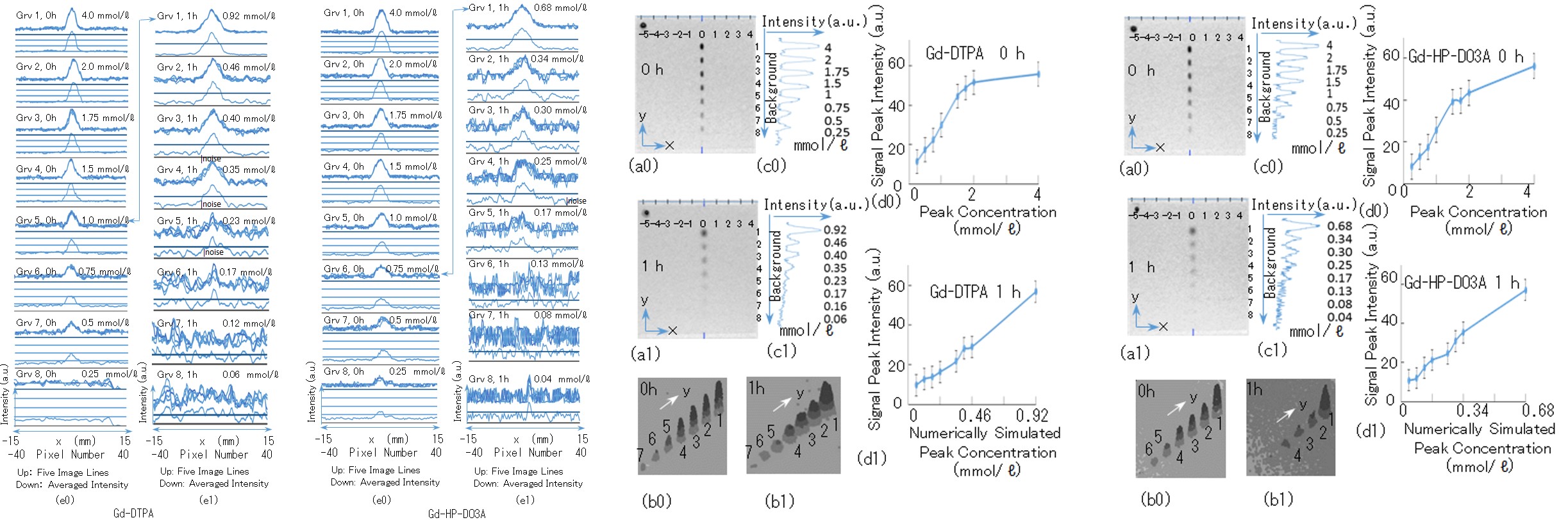
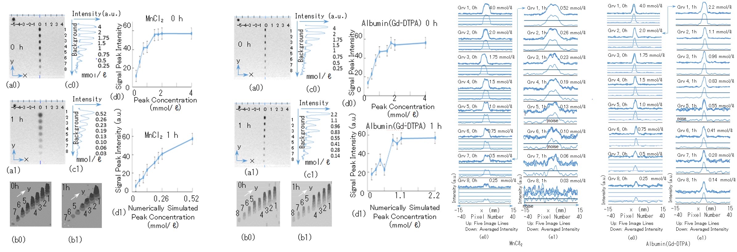
Figure 5: MRI of the eight contrast solutions added to the eight rectangular grooves on the agar gel plate at 25°C at (a0) t = 0 h and (a1) t = 1 h . The range of the x axis is from -5.0 to + 4.0 cm, and the groove numbers (Ngrv) from 1 to 8 are shown on the right side. Contour mappings of the MRI SI at (b0) t = 0 h and (b1) t = 1 h are also shown. Higher intensities correspond to higher concentrations. The eight signal peak amplitudes from Ngrv = 1 to 8 at (c0) t = 0 h and (c1) t = 1 h are displayed, with background signal levels recognized. The eight peak concentrations, in mmol/ℓ, at (c0) t = 0 h and (c1) t = 1 h are indicated on the right. The relation between the eight signal peak amplitudes and peak concentrations at (d0) t = 0 h and (d1) t = 1 h is also depicted, as well as the intensity profiles of the eight signal peaks at (e0) t = 0 h and (e1) t = 1 h. The horizontal axis goes from x = −15 to x = +15 mm. The superimposition of the five intensity profiles is shown in the upper part, and one intensity profile obtained by averaging the five profiles is shown along the five horizontal image lines as a scale in the lower part for all grooves (Ngrv = 1 to 8). Because the eight signal peaks are not normalized in (e0), the increase in the signal peak amplitude with the peak concentration can be understood in the lower part at (e0) t = 0 h. The signal peak amplitude is normalized by the peak values at the eight grooves at (e1) t = 1 h, and the line indicating half of signal intensity level between the bottom and the peak is plotted in the lower part. The bidirectional arrow between Figures 5(e0) and (e1) indicates that the lower concentration (Ngrv > 1) at t = 0 h is close to the highest peak concentration (Ngrv = 1) at t = 1 h. The ratio of the signal peak to the background noise level decreases with decreasing CA concentration at (e1) t = 1 h.

Click to enlarge

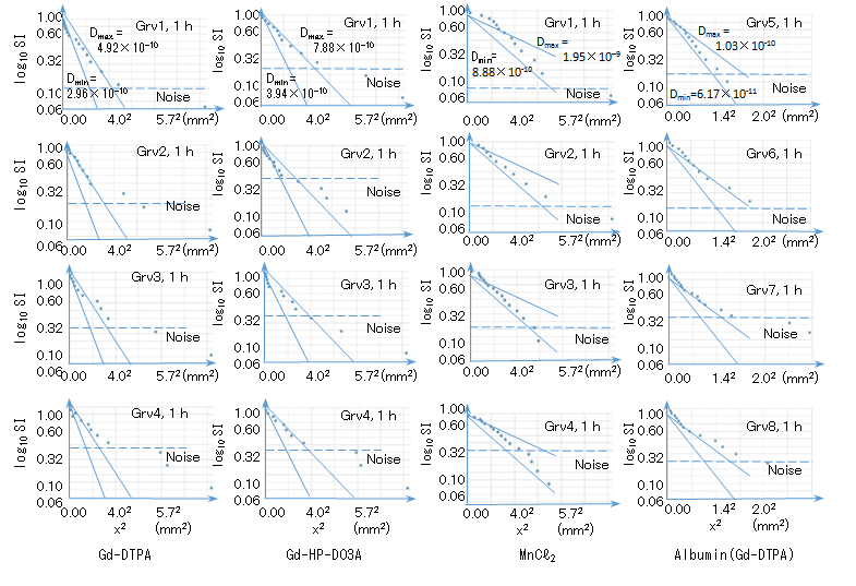
Figure 6: Intensity profiles of the signal peaks at t = 1 h. The vertical and horizontal axes are the logarithm of the intensity normalized by the peak intensity and x2, respectively. A comparison of the intensity profile indicated by the dots and the linear tail of the numerical profile shows the range of the diffusion coefficients of Gd-DTPA, Gd-HP-DO3A, and MnCℓ2 for groove numbers Ngrv from 1 to 4 and that of albumin-(Gd-DTPA) for Ngrv from 5 to 9. Because the SNR is worse for Gd-DTPA, Gd-HP-DO3A, and MnCℓ2 for Ngrv = 5 to 8, a comparison was made for Ngrv = 1 to 4. Because there is no linear relation between the signal intensity and the CA concentration at the signal peak position of albumin-(Gd-DTPA) for Ngrv = 1 to 4, a comparison was made for Ngrv = 5 to 8. The noise level is approximately 10% of the signal peaks in the highest-concentration grooves (highest raw) for the four CAs and increases up to approximately 30% of the signal peaks in the lowest-concentration grooves (lowest raw). Conclusions The diffusion coefficients of low- (MnCℓ2 (MW 126)), medium- (Gd-DTPA (MW 743) and Gd-HP-DO3 (MW 559)) and high- (albumin-(Gd-DTPA) (MW 94000)) molecular-weight MRI CAs in pure water were measured on agar gel plates at 25°C using 0.3 T spin echo proton MRI. The pixel size, NSA, and scan time were 312 µm, four, and 6 min, respectively. The agar gel plate thickness typically used for gel electrophoresis is 1 mm, and the agar concentration in pure water (18.2 MΩ·cm at 25°C) is 1.0% (w/v). Contrast solutions were prepared with the CAs and pure water, with the solution concentrations defined in terms of the paramagnetic ion concentration (PC). Eight contrast solutions with initial PCs from 0.25 mmol/ℓ to 4.0 mmol/ℓ were added to the eight rectangular grooves, 4 mm (along the phase axis) × 1 mm (along the frequency axis) in the gel plate. The Brownian motion of the CAs in water was evident in the Gaussian concentration profiles along the frequency axis. The concentration peaks decreased and the tail widths increased with time because of diffusion. The MRI signal profiles from the contrast solutions observed in the image line along the frequency axis were proportional to the PCs as a result of T1 relaxivity. When the PC is higher than the saturation concentration of approximately 1 mmol/ℓ (just above the clinical dose), the MRI signal does not increase and is saturated with the PC as a result of the T2 relaxivity. The MRI signal peak results from the CA concentration peak at the center of each groove. The relation between the signal peak and the concentration peak for each of the eight grooves was investigated at t = 0 h, just after the addition of the contrast solution (at the start of the diffusion) and at t = 1 h after the start of the diffusion. While the signal peaks were saturated in several grooves in which the initial concentration peaks exceeded the saturation concentration at t = 0 h, a linear relation between the signal peak and PC for the eight grooves for the solutions of MnCℓ2, Gd-DTPA, and Gd-HP-DO3 was confirmed at t = 1 h. The signal peaks were saturated for four grooves of the higher-concentration solutions of albumin-(Gd-DTPA) at t = 1 h, for which the concentration peak exceeded the saturation concentration and the peak part of the Gaussian signal profile collapsed because the diffusion motion of albumin-(Gd-DTPA) is the lowest among the four CAs. Thus, the MRI signals from the solutions of MnCℓ2, Gd-DTPA, and Gd-HP-DO3 and those of the solutions of albumin-(Gd-DTPA) at the four lower concentrations at t = 1 h exhibited Gaussian signal profiles that were not collapsed by signal saturation. Because Gaussian signal profiles are affected by background noise, the SNR increases with increasing CA concentration. Thus, the degree of distortion of the Gaussian signal profile increases as the CA concentration decreases. The MRI signals from the solutions of MnCℓ2, Gd-DTPA, and Gd-HP- DO3 at the four higher concentrations at t = 1 h exhibited Gaussian signal profiles, with low distortion and high SNRs. The SIs from the albumin-(Gd-DTPA) solution was the highest among those from the four CA solutions at the same PC because the T1 relaxivity of albumin-(Gd-DTPA) is the highest among the four CAs. Thus, the SIs from the solution of albumin-(Gd-DTPA) at the four lower concentrations at t = 1 h exhibited Gaussian signal profiles with low degrees of distortion and high SNRs. The Gaussian signal profiles from the four of the eight grooves for the four CA solutions were not collapsed by signal saturation and not distorted by noise, and adequate for use in the determination of the diffusion coefficients of the four CAs. The signal intensity arising from a CA is defined by eliminating background noise from the signal profile. When a horizontal line cuts across the signal profile at a certain signal intensity, the width of the signal profile is defined by the distance between the two points made by the crossing between the horizontal line and the signal profile. Although there is a linear relation between the square of the width and the logarithm of the signal intensity in the ideal Gaussian profile, the linearity deteriorates in a signal profile distorted by noise. Thus, the diffusion coefficients of the CAs determined by fitting the Gaussian concentration profiles to the observed signal profiles contain a certain amount of error. Sampling averages of five image lines, summed up along the phase axis, reduced irregularities in the signal profiles. However, the coefficient value ranges determined included measurement error of more than 10% because of the remaining irregularities due to noise. The diffusion coefficients of MnCℓ2, Gd-DTPA, Gd-HP-DO3A, and albumin-(Gd-DTPA) were determined to be (1.4 ± 0.5) × 10-9 m2/s, (0.4 ± 0.1) × 10-9 m2/s, (0.6 ± 0.2) × 10-9 m2/s, and (0.07 ± 0.02) × 10-9 m2/s, respectively. The diffusion coefficients of CAs measured in living tissue are expected to be usable diagnostics because the clinical dose concentration of MRI CAs does not induce molecular interaction and is less than 1/100 of the concentration required for diffusion coefficient measurement by means of light refractive index change. Because the diffusion coefficients of CAs are expected to be measured using gel sheets to produce standard diffusion coefficients, analytical formulae for one- dimensional diffusion from a rectangular groove were considered. The diffusion displacement of the chelate compound of paramagnetic ion for clinical use is not expected to exceed one pixel size during the typical scan time of 6 min, while that of a single paramagnetic ion such as Mn2+ is expected to exceed one pixel size because of its much higher diffusion velocity. Thus, the diffusion displacement of CAs for clinical use during a scan time of 6 min can be neglected. Because the Gaussian concentration formula is based on diffusion from an infinitely narrow source, the quasi-Gaussian concentration formula based on diffusion from a groove of finite width was approximately derived for the gel sheet experiments conducted in this study. The optimal initial CA concentration at t = 0 should be estimated, because the concentration peak in the groove should be less than the saturation concentration and because the entire concentration profile is within the range within which the MRI signal is proportional to the CA concentration at the diffusion measurement time. Thus, the quasi-Gaussian concentration formula for estimating the decrease in the peak concentration with time due to diffusion was derived as a function of the diffusion coefficient assumed before the measurement, and the results obtained with the quasi-Gaussian concentration formula were in good agreement with the exact numerical simulation results. Conducting 0.3-T MRI using a square pixel shape was not found to decrease the measurement error from over ten percent to several percent. Because the averaging of five image lines along the phase axis decreased the irregularity of the MRI signal profile along the frequency axis, decreasing the division along the phase axis, which leads to a substantial increase in the NSA, is expected to decrease the irregularity of signal profile and reduce the measurement error of the diffusion coefficient to within several percent.