Transverse and Longitudinal Hydraulic Conductivities in Hollow Fiber Dialyzer Evaluated Using Capillary Flow Analysis
<p style="text-align: justify;">A cylindrical blood dialyzer houses a hollow fiber bundle, where the dialysate inlet and outlet are located at both surface ends. The transverse and longitudinal dialysate flow paths perpendicular and parallel to the hollow fibers, respectively, could be regarded as narrow capillaries. The angle of the dialysate flow toward the central axis measured from the surface of the hollow fiber bundle after injection perpendicular to the bundle is given by the transverse-to-longitudinal hydraulic conductivity ratio κtr/κln. Because the dialysate flow paths parallel to the hollow fibers are always larger than those perpendicular, i.e., κtr/κln < 1, the dialysate fluid can only move easily along the surface of the hollow fiber bundle towards the dialysate outlet without reaching the central axis of this bundle. The transverse-to-longitudinal flow path diameter ratio was evaluated to be 0.3. Because the flow rate through the capillary was proportional to the diameter squared, κtr/κln was estimated to be 0.1, which is about the radius-to-length ratio R/L of the hollow fiber bundle. Current dialyzers were considered to allow the dialysate flow to reach the central axis of the hollow fiber bundle because they satisfy κtr/κln ≥ R/L. Slight decreases in the hollow fiber density were expected to provide distinct increases in κtr/κln and dialysis efficiency by allowing the dialysate flow to reach the central axis while maintaining a comparatively low increase in the fiber bundle’s diameter.</p>
Introduction
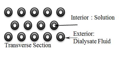
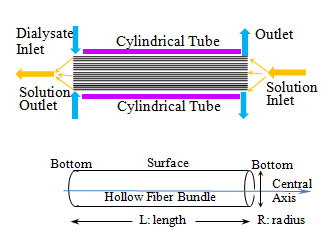
Porous media include void fractions consisting of narrow gaps whose volume ratio is called the porosity φ. When a pressure gradient is generated in porous media, a permeable flow occurs in accordance with Darcy’s law, where the flow rate is proportional to both the hydraulic conductivity and pressure gradient [1]. Permeable flow analyses have been used in liquid chromatography [2] and the performance evaluations of heterogeneous porous materials [3]. A hollow fiber dialyzer is a typical application of a fibrous porous media [4]. Blood dialysis is carried out using hollow fiber membranes whose external surfaces are the flow paths of the dialysate fluid composed of saline while blood flows through the internal sections of the hollow fibers, as shown in Figures 1 and 2 [5]. A bundle of 10,000 hollow fibers is housed in the cylindrical dialyzer tube. The surface of the cylindrical hollow fiber bundle consists of one circular surface and two flat circular bottoms at the ends. The dialysate inlet and outlet are located on the surface at the opposite ends of the hollow fiber bundle with a width of 10 mm. The blood inlet and outlet are located at the opposite bottoms of the hollow fiber bundle. The anisotropic hydraulic conductivities—the longitudinal (κln) and transverse (κtr) hydraulic conductivities parallel and perpendicular to the fibers, respectively—characterize the permeable flow through the hollow fiber bundle as fibrous and porous [6].
Lower: Schematic of a hollow fiber bundle composed of a circular side surface and two flat bottoms. The radius-to- length ratio R/L is 0.1.
The dialysate flow rate at the dialysate inlet of the hollow fiber bundle is determined by κtr because the dialysate flow is perpendicular to the hollow fiber bundle. Thus, the length L and radius R of the hollow fiber bundle are empirically determined to be about 200 mm and 20 mm, respectively, where the radius-to-length ratio R/L is 0.1. The angle of the dialysate flow toward the central axis measured from the surface of the hollow fiber bundle just after injection into the bundle is given by the transverse- to-longitudinal hydraulic conductivity ratio κtr/κln. If κtr/κln ≥ R/L, the dialysate flow can reach the deep region along the central axis of the hollow fiber bundle after injection at the dialysate inlet [6]. If κtr/κln < R/L, the dialysate flow has difficulty reaching the central axis of the hollow fiber bundle. As a result, the dialysate fluid mainly flows on the surface of the hollow fiber bundle to the outlet. Although velocity encoding during proton magnetic resonance imaging (MRI) can observe the uniformity in the dialysate flow at a cross section at the midpoint of the length of the hollow fiber bundle, the dialysate flow cannot reach the central axis of the bundle just after injection at the surface of the bundle because the dialysate flow is first injected perpendicular to the hollow fibers and it is much easier for the dialysate fluid to flow parallel to them [5, 6]. Although the MR contrast solution injected into the dialysate flow revealed that the dialysate flow almost reached the deep region with no localizations around the surface of the hollow fiber bundle, evidence of the possibility of the dialysate flow reaching the central axis of the bundle is required for the effective use of this region. The aim of this research is to confirm that the dialysate flow reaches this region, i.e., the condition κtr/κln ≥ R/L is almost satisfied in current dialyzers, and to provide useful formulas for designs to improve the dialysis efficiency with effective utilization of the entire volume of the hollow fiber bundle, where the fiber (packing) density fb (=1 – φ) and R/L are about 0.5 and 0.1, respectively, as inferred from current dialyzers [7].
Pressurized Flow in Circular and Slab Capillaries as a Model of Dialysate Flow
By regarding the fiber bundle as a regular array of parallel solid cylinders, κln and κtr for water flowing through fiber bundles have been analyzed [8]. Analytical formulas were derived using a series expansion in a way similar to the derivation of Stokes’ law [9]. Although the analytical formulas are strict and adaptable to a wide range of fiber densities, they are complex and lacking in terms of providing a practical picture. Concise practical formulas for the anisotropic hydraulic conductivities are required for an efficient design of the entire volume of a hollow fiber bundle. Because the Poiseuille flow (PF) formula is a useful reference for evaluating the flow rate of the pressurized flow in a capillary [9, 10, 11, 12], the permeable flow analyses in this research will be based on PF. A central vertical section of the cylindrical tube of the dialyzer is schematically depicted in Figure 1. The inlet and outlet ports of the dialysate flow path are located at the left and right ends of the dialyzer, respectively, and those of the blood flow are located at the right and left ends of the dialyzer, respectively. The inlet and outlet ports of the dialysate flow path are located on the hollow fiber bundle surface at opposite ends of the dialyzer and surround the surface ends having a width of 1.0 cm along the bundle axis direction. The transverse section of the hollow fiber bundle is schematically depicted in Figure 2. The hollow fiber has an inner diameter and membrane thickness of 210 and 30 µm, respectively. The interior and exterior of the hollow fiber consist of blood and dialysate compartments, respectively. The dialysate flow path is the inter-hollow-fiber space spreading over the external surfaces of the hollow fiber. A vast number of thin flow paths consist of gaps between narrow fibers. In order to analyze the thin flow paths, two stationary flow profiles— the PF and two-dimensional Poiseuille flow (2DPF)—are useful references because they are analytical solutions. The PF and 2DPF are generated by a pressure gradient (pressurized flow) in circular (Figure 3) and slab (Figure 4) capillaries, respectively.
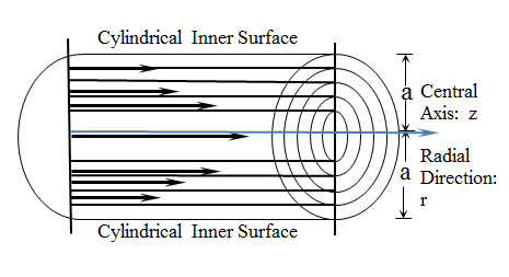
Figure 3: Cylindrical laminar flow layers in a circular capillary surrounded by a cylindrical surface. A pressure gradient ∂p/∂z uniformly added throughout the circular cross section generates cylindrical laminar flow layers. The laminar flow velocities in the regions closest to the inner surface and central axis of the cylindrical capillary are low and high, respectively.
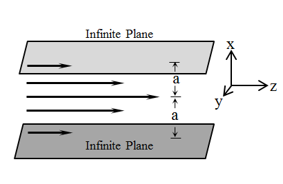
Figure 4: Planar laminar flow layers in a slab capillary surrounded by two infinite planes. A pressure gradient ∂p/∂z is applied uniformly throughout the slab cross section, generating planar laminar flow layers. The laminar flow velocities in the regions closest to the inner surface and central plane of the slab capillary are low and high, respectively.
The PF is generated in a circular linear capillary with an infinite straight length, as shown in Figure 3. The cylindrical coordinates are r in the radial direction perpendicular to the central axis of the circular capillary and z along the central axis. Because uniformity along the axial direction is assumed, the static pressure of the fluid p(z) is uniform throughout the cross section and varies linearly with the axial displacement, and the pressure gradient $\partial p(z)/\partial z$ is uniform throughout the cross section and does not vary with the axial displacement. With the assumption of laminar flow conditions, $c u_z(r)$ is induced by $\partial p/\partial z$, has only an axial direction component, is a function of the radial displacement, and does not depend on the axial displacement. Because the inner diameter of the circular capillary is $2^c a$, the inner surface of the capillary is located at $r = c a$. Growth of the PF was simulated according to the Navier–Stokes fluid equation with cylindrical geometry:
$$\rho \frac{\partial^c u_z}{\partial t} = \mu \frac{1}{r} \frac{\partial}{\partial r} \left( r \frac{\partial^c u_z}{\partial r} \right) - \frac{\partial p}{\partial z}, \quad 0 \leq r \leq c a$$ (2.1)
where $\rho$ and $\mu$ are the density and viscosity of the Newtonian fluid, respectively; and $t$ is the time. The convective term $c u \cdot \nabla$ $c u_z$ has been omitted assuming that the laminar flow conditions are $c u_z = 0$, $c u_\theta = 0$, $\partial/\partial \theta = 0$, and $\partial/\partial z = 0$, where $\theta$ is the azimuthal angle. The no-flow boundary on the inner surface is expressed as $c u_z(r) = 0$ at $r = c a$ and $0 \leq t$. $\partial p/\partial z$ is applied after $t = 0$. The solution of Equation (2.1) leads to the growth of the PF over time:
$$c u(r,t) = \frac{1}{4 \mu} \frac{\partial p}{\partial z} \left\{ \left( c a^2 - r^2 \right) - 8 c a^2 \sum_{n=0}^{\infty} \frac{J_0 \left( \frac{K_n r}{c a} \right)}{\kappa_n^3 J_1 \left( \kappa_n \right)} \exp \left( - \frac{K_n^2 v t}{c a^2} \right) \right\}$$ (2.2)
where $v = \mu/\rho$, $J_0$ is the 0th-order Bessel function, and $K_n$ is a zero point of the Bessel function satisfying $J_0(K_n) = 0$ and $K_n > 0$ [10]. The growth period $t_g PF$ of the PF is defined as [12]:
$$t_g PF = \frac{5 c a^2}{2.4^2 v}$$ (2.3)
When $t > t_g PF$, the maximum of the exponential term in Equation (2.2) becomes less than 0.0067, where $J_0(2.4) = 0$ and $\exp(-5.0) = 0.0067$ are used. When $t > t_g PF$, $c u_z(r)$ from Equation (2.2) approaches a parabolic flow profile in the steady state:
$$c u_z(r) = \frac{1}{4 \mu} \frac{\partial p}{\partial z} \left( c a^2 - r^2 \right), \quad 0 \leq r \leq c a$$ (2.4)
The flow velocity $c u_z, a v$, which is averaged over the entire transverse cross section of the circular capillary, is defined as $c u_z, a v = \int_0^c a c u_z(r) 2 \pi r dr / \int_0^c 2 \pi r dr$ and is calculated to be:
The 2DPF is generated in a rectangular linear capillary with an infinite straight length, as shown in Figure 4. Because the rectangular capillary approaches a slab volume surrounded by two parallel plates situated horizontally with an infinite area separated by a distance of $2^c a$ in the limit of infinite extension of the two horizontal sides in the rectangular cross section, the rectangle capillary is called a slab capillary. The origin of the three-dimensional Cartesian coordinates is located at the central position between the two plates, where $x$ is in the direction perpendicular to the two horizontal plates, and $y$ and $z$ are in the plane of the two plates. The central axis and the cross section of the slab capillary are the $z$ axis and the $x-y$ plane, respectively. The radial direction of the slab capillary is in the $x$ direction. With the assumption of laminar flow conditions, $c u_z(r)$ has only an axial direction component, is a function of the radial displacement, and does not depend on the axial displacement. Because the inner diameter of the slab capillary is $2^c a$, the inner surface of the capillary is located at $x = c a$. The growth of the 2DPF was simulated according to the Navier–Stokes fluid equation with the slab geometry:
$$\rho \frac{\partial^c u_z}{\partial t} = \mu \frac{\partial^2 u_z}{\partial x^2} - \frac{\partial p}{\partial z}, \quad 0 \leq x \leq s a$$ (2.6)
The no-flow boundary on the inner surface is expressed as $s u_z(x) = 0$ at $x = s a$ and $0 \leq t$. $\partial p / \partial z$ is applied after $t = 0$.
The solution of Equation (2.6) leads to the growth of the 2DPF over time:
$$s u(y,t) = \frac{1}{2 \mu} \frac{\partial p}{\partial z} \left[ \left( s^2 - x^2 \right) - 4 s^2 \sum_{n=0}^{\infty} (-1)^n \frac{\cos \left\{ \left( n \pm \frac{1}{2} \right) \frac{\pi x}{s a} \right\}}{\left( n \pm \frac{1}{2} \right)^3 \pi^3} \exp \left\{ - \left( n \pm \frac{1}{2} \right)^2 \frac{\pi^2 v t}{s a^2} \right\} \right]$$ (2.7)
The growth period $t_{g,2DPF}$ of the 2DPF is defined as
$$t_{g,2DPF} = \frac{20 s^2}{\pi^2 v}$$ (2.8)
When $t > t_{g,2DPF}$, the maximum of the exponential term in Equation (2.7) becomes less than 0.0067, where $\cos(\pi/2) = 0$ and $\exp(-5.0) = 0.0067$ are used. When $t > t_{g,2DPF}$, $s u_z(r)$ from Equation (2.7) approaches the steady-state parabolic flow profile expressed as
$$s u_z(x) = \frac{\partial p}{\partial z} \frac{1}{2 \mu} \left( s^2 - x^2 \right) \left( -s a \leq x \leq s a \right)$$ (2.9)
The flow velocity $s u_z_{ave}$, which is averaged over the transverse cross section of the slab capillary for a one-unit transverse distance in the $x$ direction, is defined as
$$s u_z_{ave} = \frac{\int_{-s a}^s s u_z(x) dx}{\int_{-s a}^s dx}$$ (2.10)
and calculated to be
Transverse and Longitudinal Hydraulic Conductivities Evaluated Using Capillary Flow Analysis
Fiber Density and Permeable Flow Analysis in Circular and Square Fiber Bundles
As a model of the hollow-fiber bundle consisting of straight fibers, we consider an infinite linear bundle of circular and square fibers whose cross sections are shown in Figures 5 and 6, respectively, where the flow path (flow-allowed region) and rigid space (flow-inhibited region) are the outside and inside of the fibers. Because the hollow fibers are flexible materials and do not always have accurate circular cross sections owing to fins and windings, they cannot be modeled as strictly solid cylinders. Therefore, bundles of circular and square hollow fibers, as shown in Figures 5-7, are considered to be an adequate model instead of regular arrays of parallel solid cylinders. The cross section of the circular fiber has a diameter of $2^2 a$, as shown in Figure 5.
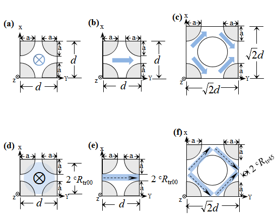
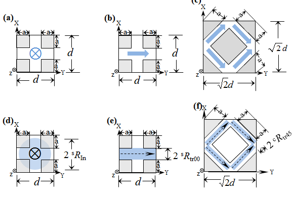
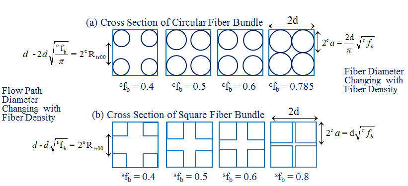
Figure 7: Cross sections of (a) circular and (b) square fiber bundles changing with the fiber density. The square fiber density is higher than the circular fiber density for the same transverse flow path diameter Rtr. Formulas for the fiber diameters 2ca and 2sa and the flow path diameters 2cRtr00 and 2sRtr00 are shown on the right and left sides, respectively.
One side of the cross section of the square fiber has a length of 2sa, as shown in Figure 6. Because the circular and square fibers are regularly arranged, where the minimum interval between the fibers is d, there is a periodic unit cell cube whose side length and surface plane area are d and d2, respectively. Hereafter, variables related to the circular and square fiber bundles are denoted by the superscripts c and s preceding the variable, respectively. In the circular and square fiber bundles, the three-dimensional Cartesian coordinates are x and y in the transverse direction perpendicular to the fibers and z in the longitudinal direction parallel to the fibers. Uniformity along the z coordinate is assumed. The fiber (flow-inhibited) densities cfb and sfb in the circular and square fiber bundles whose cross sections are shown in Figures 5a and 6a, respectively are a π
2 c $$ ^ {\mathrm {c}} \mathrm {f} _ {\mathrm {b}} = \frac {\pi^ {\mathrm {c}} a ^ {2}}{\mathrm {d} ^ {2}}, (0 \leq^ {\mathrm {c}} \mathrm {f} _ {\mathrm {b}} \leq \frac {\pi}{4}) $$ b c 2 b c
2 s $$ ^ {\mathrm {s}} \mathrm {f} _ {\mathrm {b}} = \frac {4 ^ {\mathrm {s}} a ^ {2}}{\mathrm {d} ^ {2}}, (0 \leq^ {\mathrm {s}} \mathrm {f} _ {\mathrm {b}} \leq 1) \tag {3.1} $$ a b s 2 b s The changes in the cross sections of the circular and square fiber bundles as functions of the fiber density are shown in Figure. 7, where the fiber density ranges from 0.4 to 0.8, and the formulas for the fiber diameters 2ca and 2sa derived from Equation (3.1) are shown on the right side. In the circular fiber bundle, the maximum fiber density is determined as cfb = π/4 (≒0.785) at ca = d/2, where the surfaces of adjacent fibers touch each other, and the minimum is cfb = 0 at ca = 0. In the square fiber bundle, the maximum fiber density sfb is 1.0 at sa = d/2 and the minimum is sfb = 0 at sa = 0. The porosities (flow area density) of cg and sg in the cross sections of the circular and square fiber bundles are related to cfb and sfb as cg + cfb = 1 and sg + sfb = 1, respectively. When there is a gradient in p along the x, y, and z directions, an average flow velocity uave is generated along it. uave is defined in the periodic unit cell. u(x, y) is set to zero in the rigid region and does not change with the longitudinal displacement. In Darcy’s law, the hydraulic conductivity κ appears as a proportional coefficient relating $\nabla p$ and $u_{\text{ave}}$ as $u_{\text{ave}} = \kappa \nabla p$. The longitudinal and transverse flow velocities are averaged over the cross sectional area $d^2$ of the periodic unit cell. The longitudinal and transverse average flow velocities $u_{\text{inave}}$ and $u_{\text{trave}}$ are related to $\kappa_{\text{in}}$ and $\kappa_{\text{tr}}$, respectively, as [1, 6].
$$u_{\text{tr,ave}} = \kappa_{\text{tr}} \cdot \frac{\partial p}{\partial r}, \quad r = x, y,$$
$$u_{\text{in,ave}} = \kappa_{\text{in}} \cdot \frac{\partial p}{\partial z},$$
(3.2)
where $r$ is the direction in the $x-y$ plane, and $\partial p/\partial r$ are the pressure gradients in the longitudinal and transverse directions parallel and perpendicular to the fiber bundle, respectively. Because the flow profiles in the complicated flow paths in Figures 5 and 6 cannot be obtained analytically, the average flow velocity through the fiber bundle can be evaluated by referring to the parabolic flow profiles in Equations (2.4) and (2.9).
Although only one flow pattern is allowed for the longitudinal flow parallel to the fiber, as shown in Figures 5a and 6a for the circular and square fibers, respectively, various flow patterns are allowed for the transverse flow perpendicular to the fiber bundle. The transverse flow pattern changes according to the incident angle at the unit cell. At each 90° interval in the incident angle, similar flow patterns appear repeatedly from the symmetry. Therefore, two types of transverse flow patterns are adopted as typical flow patterns; one at 0° incidence, as shown in Figures 5b and 6b, and the other at 45° incidence, as shown in Figures 5c and 6c. The longitudinal hydraulic conductivities parallel to the circular and square fibers are denoted by $c_{\text{tr}}$ and $s_{\text{tr}}$, respectively. The transverse hydraulic conductivities perpendicular to the circular and square fibers are denoted by $c_{\text{tr}}^{00}$, $c_{\text{tr}}^{45}$, and $s_{\text{tr}}^{00}$, $s_{\text{tr}}^{45}$, respectively, where the 0° and 45° incidences are denoted by the superscripts 00 and 45, respectively. One longitudinal hydraulic conductivity $k_{\text{in}}$ and two transverse hydraulic conductivities $k_{\text{tr}}^{00}$, $k_{\text{tr}}^{45}$ will be evaluated analytically.
**Longitudinal Hydraulic Conductivity by Regarding the Longitudinal Flow Path as a Circular Capillary**
Consider longitudinal flow paths parallel to the circular and square fiber bundles as shown in Figures 5a and 6a. The longitudinal flow paths outside the circular and square fibers can be replaced by virtual circular capillaries whose inner diameters are determined by the area equivalence that the cross-sectional area of the virtual circular capillary is the same as that of the longitudinal flow path in the unit cell area $d^2$, i.e.,
$$\pi c R_{\text{in}}^2 + \pi c a^2 = d^2,$$
$$\pi c R_{\text{in}}^2 + 4 c a^2 = d^2.$$
(3.3)
Therefore, the longitudinal flow path diameters, $2 c R_{\text{in}}$ and $2 c R_{\text{in}}$, of the virtual circular capillaries are determined from $c_{\text{tr}}$ and $s_{\text{tr}}$ using Equations (3.1) and (3.3) as:
$$2 c R_{\text{in}} = 2 \sqrt{\frac{1 - c^2 f_b}{\pi}} \cdot d,$$
$$2 s R_{\text{in}} = 2 \sqrt{\frac{1 - s^2 f_b}{\pi}} \cdot d.$$
(3.4)
The changes in $2 c R_{\text{in}}$ and $2 s R_{\text{in}}$ as a function of the fiber density in the circular and square fiber bundles are plotted in Figure 8a. The circular cross sections of the virtual circular capillaries are indicated by the grey circles in Figures 5d and 6d. The average flow velocity through the virtual circular capillary can be evaluated with the aid of the PF formula in Equation (2.5). Substituting $c_{\text{tr}}$ and $s_{\text{tr}}$ into Equation (2.5), the longitudinal average flow velocities $c_{\text{tr}}$ and $s_{\text{tr}}$ in the virtual circular capillary are calculated as $c_{\text{tr}}$ and $s_{\text{tr}}$ = $(dp/dz)(c_{\text{tr}}^2/8\mu)$ and $s_{\text{tr}}$ and $s_{\text{tr}}$ = $(dp/dz)(c_{\text{tr}}^2/8\mu)$, respectively, where $dp/dz$ is the pressure gradient in the longitudinal direction parallel to the fiber bundle expressed in Equation (3.2). Because $c_{\text{tr}}$ and $s_{\text{tr}}$ are averaged over the circular cross sections $\pi R_{\text{in}}^2$ and $\pi R_{\text{in}}^2$, respectively, $c_{\text{tr}}$ and $s_{\text{tr}}$ should be multiplied by the factors $(\pi c R_{\text{in}}^2/d^2)$ and $(\pi R_{\text{in}}^2/d^2)$, respectively, to obtain the average velocities $c_{\text{tr}}$ and $s_{\text{tr}}$ where averaging is performed over the sectional area $d^2$ of the periodic unit cell cube. Thus, we obtain the following from Equation (2.5):
$$c_{\text{tr}} = \frac{dp}{dz} - \frac{c R_{\text{in}}^2}{8\mu} \pi c R_{\text{in}}^2$$
$$s_{\text{tr}} = \frac{dp}{dz} - \frac{s R_{\text{in}}^2}{8\mu} \pi s R_{\text{in}}^2$$
(3.5)
Which are averaged in the unit cell and are necessary for evaluating the longitudinal hydraulic conductivity. Using Equations (3.1), (3.2), (3.4), and (3.5), $c_{\text{tr}}$ and $s_{\text{tr}}$ in the virtual circular path assumed in the circular and square fiber bundles, as shown in Figures 5d and 6d, respectively, are derived as:
Copyright © Osuga T, et al.
( ) ⋅ ⋅
, 4 π ≦ f ≦ 0.0 d f 1- 8
$$ ^ {\mathrm {c}} \kappa_ {\ln} = \frac {1}{8 \pi u} $$
b 2 2 b c ln c πμ
( ) ( ) ) 6.3 ( 1.0 ≦ f ≦ 0.0 d f 1- 8π
$$ ^ {\mathrm {s}} \kappa_ {\ln} = \frac {1}{8 \pi l} $$
b 2 2 b s ln s ⋅ ⋅
μ cκln and sκln in Equation (3.6) are similar, except for the difference that the upper limits of the fiber density are cfb = π/4 and sfb = 1.0 in the circular and square fiber bundles, respectively.
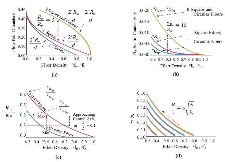
(b) Dependence of the longitudinal κln and transverse κtr hydraulic conductivities in square and circular fiber bundles on the fiber density. The maximum fiber densities of the square and circular fiber bundles are 1.0 and π/4, respectively. Although the longitudinal hydraulic conductivity is similar in both the square and circular fiber bundles, the transverse hydraulic conductivity in the square fiber bundle is greater than that in the circular fiber bundle at the same fiber density.
(c) The transverse-to-longitudinal hydraulic conductivity ratio κtr/κln in the square and circular fiber bundles as functions of the fiber density. κtr/κln ranges from a minimum in the circular fiber bundle to a maximum in the square fiber bundle and involves the radius-to-length ratio R/L = 0.1 around the practical fiber density fb ≒ 0.5. The ratio κtr/κln ≒ 0.1 at fb ≒ 0.5 is estimated from (Rtr/Rln)2 ≒ 0.1 at fb ≒ 0.5.
(d) R/L of the hollow fiber bundle is proportional to fb-0.5, where the radius a = ca, sa and the total number of hollow fibers N is constant. When R/L is 0.1 at fb = 0.4, 0.5, 0.6, 0.7, and 0.8, R/L increases as fb decreases when L and N are constant. Because a slight decrease in fb yields a distinct increase in κtr/κln and a slight increase in R/L, a slight decrease in fb will lead to distinctly effective utilization in the deep region of the hollow fiber bundle with a slight increase in R.
Transverse Hydraulic Conductivity by Regarding the Transverse Flow Path as a Slab Capillary at 0° Incidence
Consider transverse flow paths perpendicular to the circular and square fiber bundles at 0° incidence as shown in Figures 5b and 6b. Quantities related to 0° incidence are denoted with the subscript 00. The transverse flow paths for the circular and square fiber bundles in the unit cell can be replaced by a virtual slab capillary whose inner diameters $2^{c}R_{tr00}$ and $2^{s}R_{tr00}$ are set according to
$$2^{c}R_{tr00} + 2^{c}a = d,$$
$$2^{s}R_{tr00} + 2^{s}a = d. \tag{3.7}$$
Therefore, $2^{c}R_{tr00}$ and $2^{s}R_{tr00}$ of the virtual slab capillaries are determined from $cf_b$ and $sf_b$ from Equations (3.1) and (3.7) as
$$2^{c}R_{tr00} = d - 2d\sqrt{\frac{cf_b}{\pi}},$$
$$2^{s}R_{tr00} = d - d\sqrt{sf_b} \tag{3.8}$$
These equations are shown on the left hand side of Figure 7. The changes in $2^{c}R_{tr00}, 2^{s}R_{tr00}$ as functions of the fiber density in the circular and square fiber bundles are plotted in Figure 8a. Cross sections of the virtual slab capillaries are indicated by grey rectangles in Figures 5e and 6e. The average flow velocity in the virtual slab capillary can be evaluated with the aid of the 2DPF formula in Equation (2.10). Substituting $R_{tr00}$ and $sR_{tr00}$ into Equation (2.10), the transverse average flow velocities $c_{tr00,ave}'$ and $s_{tr00,ave}'$ in the virtual slab capillary are calculated as $c_{tr00,ave}' = (dp/dr)(c_{tr00}^2/3\mu)$ and $s_{tr00,ave}' = (dp/dr)(s_{tr00}^2/3\mu)$, respectively, where dp/dr is the pressure gradient in the transverse direction perpendicular to the fiber bundle in Equation (3.2). Because $c_{tr00,ave}'$ and $s_{tr00,ave}'$ are averaged over the slab cross sections $2^{c}R_{tr00}d$ and $2^{s}R_{tr00}d$, respectively, where $d$ is the depth of the unit cell, the factors $(2^{c}R_{tr00}d/d^2)$ and $(2^{s}R_{tr00}d/d^2)$ should be multiplied by $c_{tr00,ave}'$ and $s_{tr00,ave}'$, respectively, to obtain the average velocities $c_{tr00,ave}$ and $s_{tr00,ave}$, where averaging is performed over the sectional area $d^2$ in the periodic unit cell cube. Thus, we obtain the following from Equation (2.10):
$$c_{tr00,ave} = \frac{dp}{dz} \cdot \frac{cR_{tr00}}{3\mu} \cdot \frac{2^{c}R_{tr00}}{d},$$
$$s_{tr00,ave} = \frac{dp}{dz} \cdot \frac{sR_{tr00}}{3\mu} \cdot \frac{2^{s}R_{tr00}}{d} \tag{3.9}$$
which are averaged in the unit cell and are necessary for evaluating the transverse hydraulic conductivity. Using Equations (3.1), (3.2), (3.8), and (3.9), the transverse hydraulic conductivities $c_{tr00}$ and $s_{tr00}$ at 0° incidence in the virtual slab paths assumed in the circular and square fiber bundles in Figures 5e and 6e, respectively, are derived as
$$c_{cr}^{00} = \frac{1}{12\mu} \cdot \left(1 - 2\sqrt{\frac{cf_b}{\pi}}\right)^3 d^2 \quad (0.0 \leq cf_b \leq \frac{\pi}{4}),$$
$$s_{cr}^{00} = \frac{1}{12\mu} \cdot \left(1 - \sqrt{sf_b}\right)^3 d^2 \quad (0.0 \leq sf_b \leq 1.0) \tag{3.10}$$
Transverse Hydraulic Conductivity by Regarding the Transverse Flow Path as a Slab Capillary at 45° Incidence
Consider transverse flow paths perpendicular to the circular and square fiber bundles at 45° incidence as shown in Figures 5c and 6c, where the cross section of one periodic unit cell is $(\sqrt{2}d)^2$. Quantities related to 45° incidence are denoted with the subscript 45. The transverse flow paths for the circular and square fiber bundles in the unit cell can be replaced by two virtual slab capillaries whose inner diameters are set according to
$$2(2^{c}R_{tr45}) + 4a = 2d,$$
$$2(2^{c}R_{tr45}) + 4a = 2d \tag{3.11}$$
Therefore, the transverse flow path diameters $2^{c}R_{tr45}$ and $2^{s}R_{tr45}$ of the virtual slab capillaries are determined from $cf_b$ and $sf_b$ using Equations (3.1) and (3.11) as
$$2^{c}R_{tr45} = d - 2d\sqrt{\frac{cf_b}{\pi}},$$
$$2^{s}R_{tr45} = d - d\sqrt{sf_b} \tag{3.12}$$
The cross sections of the virtual slab capillaries are indicated by the grey rectangles in Figures 5f and 6f. The transverse flow velocity is averaged over the cross-sectional area $(\sqrt{2} d)^2$ of the periodic unit cell. The average flow velocity in the virtual slab capillary can be evaluated with the aid of the 2DPF formula in Equation (2.10). Substituting $c_{tr45}$ and $s_{tr45}$ into Equation (2.10), the transverse average flow velocities $c_{tr45,ave'}$ and $s_{tr45,ave'}$ in the virtual slab capillary are calculated as $c_{tr45,ave'} = (dp/dr)(c_{tr45}^2/3\mu)$, $s_{tr45,ave'} = (dp/dr)(s_{tr45}^2/3\mu)$, respectively, where $dp/dr$ is the pressure gradient in the transverse direction perpendicular to the fiber bundle in Equation (3.2). Because $c_{tr45,ave'}$ and $s_{tr45,ave'}$ are the velocities averaged over the slab cross sections 4$c_{tr45}$d and 4$s_{tr45}$d, respectively, where $d$ is the depth of the unit cell, the factors $(4c_{tr45}d/\sqrt{2} d^2)$ and $(4s_{tr45}d/\sqrt{2} d^2)$ should be multiplied by $c_{tr45,ave'}$ and $s_{tr45,ave'}$, respectively, to obtain the average velocities $c_{tr45,ave'}$ and $s_{tr45,ave'}$ where averaging is performed over the cross-sectional area $(\sqrt{2} d)^2$ in the periodic unit cell cube. Because the two flow paths in Figures 5c and 6c have an oblique angle of 45° relative to the side of a unit cell having a length of $\sqrt{2} d$, the actual pressure gradient should be reduced by a factor of $1/\sqrt{2}$. Thus, we obtain the following from Equation (2.10):
$$c_{tr45,ave} = \frac{dp}{dz} \cdot \frac{c_{tr400}}{3\mu} \frac{4c_{tr45}}{(\sqrt{2} d)} \frac{1}{\sqrt{2}},$$
$$s_{tr45,ave} = \frac{dp}{dz} \cdot \frac{c_{tr400}}{3\mu} \frac{4s_{tr45}}{(\sqrt{2} d)} \frac{1}{\sqrt{2}}$$
which are averaged within the unit cell and are necessary for evaluating the transverse hydraulic conductivity. Using Equations (3.1), (3.2), (3.12), and (3.13), the transverse hydraulic conductivities $c_{tr45}$ and $s_{tr45}$ at 45° incidence in the virtual slab paths assumed in the circular and square fiber bundles shown in Figures 5f and 6f, respectively, are derived as
$$c_{cr}^{45} = \frac{1}{12\mu} \left( 1 - 2 \sqrt{\frac{c_{f_b}}{\pi}} \right)^3 d^2 \left( 0.0 \leq c_{f_b} \leq \frac{\pi}{4} \right),$$
$$s_{cr}^{45} = \frac{1}{12\mu} \left( 1 - \sqrt{\frac{c_{f_b}}{\pi}} \right)^3 d^2 \left( 0.0 \leq c_{f_b} \leq 1.0 \right)$$
The transverse hydraulic conductivities at 0° and 45° incidence in Equations (3.10) and (3.14) are similar for both the circular and square fiber bundles as functions of $c_{f_b}$ and $s_{f_b}$.
Efficient Dialysate Flow Path Determined by the Transverse-to-Longitudinal Hydraulic Conductivity Ratio
The Validity of Regarding the Permeable Flow through A Hollow Fiber Bundle as Poiseuille Flow through Capillaries
Because there is a single hollow fiber located at each cross section $d^2$ of one periodic unit cell in the hollow fiber bundle, the cross section $\pi R^2$ of the hollow fiber bundle and the number of the hollow fiber bundles $N$ are related as $\pi R^2 = Nd^2$. For typical values of $N = 10^4$ and $R = 20$, $d$ is 350 $\mu$m using this relationship. Because a typical value of the exterior diameter of the hollow fiber is 250 $\mu$m, the width of the gap between the hollow fibers is about 100 $\mu$m. Thus, the inner diameter of the virtual capillary created by the gap between hollow fibers is on the order of 100 $\mu$m ($= 350 \mu$m – 250 $\mu$m). Therefore, the growth periods for the PF and 2DPF inside the capillary are estimated to be several tens of milliseconds from Equations (2.3) and (2.8) [10, 11, 12]. Because these growth periods are very small, the assumption of a stationary laminar flow for the dialysate flow when deriving the longitudinal and transverse hydraulic conductivities in Equations (3.6), (3.10), and (3.14) is considered to be valid. In addition, the assumption requires a lower Reynolds number $Re = \rho U_c L_c/\mu$ for the dialysate flow, where $U_c$ and $L_c$ are the characteristic velocity and length, respectively.
The cross section $S$ of the dialysate flow path in the hollow fiber bundle is given by $S = \pi R^2 (1 - f_b)$. Because $S = 6.3 \text{ cm}^2$, the average dialysate flow velocity $U$ along the axial direction is 1.3 cm/s for a dialysate flow rate of 500 ml/min and $f_b = 0.5$. The density and viscosity of the dialysate fluid at 37.0 °C are $0.994 \times 10^3 \text{ kg/m}^3$ and $0.725 \times 10^{-3} \text{ Pa}$, respectively. For $L = 100 \mu$m, which is the external radius of the hollow fiber, $Re = 1.3$ at 37 °C. Although $L$ will extend to ten times the external radius, the Reynolds number is expected to reach 10 as a maximum. Although weak stationary vortex generation is expected at $Re = 10$, the dialysate flow through the hollow fiber bundle is estimated to be a laminar stationary flow. Therefore, the assumption of a stationary laminar flow is valid, and the average flow through the hollow fiber bundle can be evaluated on the basis of the PF formulas in Equations (2.4) and (2.9).
Possibility of Dialysate Fluid Reaching the Deep Region in the Hollow Fiber Bundle
Because the hollow fibers are flexible materials with fins and windings, they cannot be strictly modeled as solid cylinders. Therefore, bundles of circular and square fibers, as shown in Figures 5-7, are considered to be an adequate model for representing a practical hollow fiber bundle instead of considering regular arrays of parallel solid cylinders. The changes in the cross sections of the square and circular fiber bundles are shown in Figure 7 as functions of cfb and sfb. cRln,v and sRln,v in Equation (3.4) and cRtr00, sRtr00, cRtr45, and sRtr45 in Equations (3.8) and (3.12) are plotted as functions of cfb and sfb in Figure 8a. The maximum fiber densities are 1 and π/4 (=0.785) for the square and circular fiber bundles, respectively, where the fibers contact each other. The minimum fiber densities are 0 for both the square and circular fiber bundles. Although a longitudinal flow path remains in a circular fiber bundle at the maximum fiber density fb = π/4, the transverse flow path is completely closed at this density in both circular and square fiber bundles. The transverse- to-longitudinal flow path diameter ratio Rtr/Rln is about 0.3 around the practical fiber density fb ≒ 0.5. The longitudinal and transverse flow velocities are proportional to the square of the capillary radius, as shown in Eqs. (2.2) and (2.4). Therefore, κtr/κln is estimated to be about 0.1 around the practical fiber density fb ≒ 0.5, because (Rtr/Rln)2 ≒ 0.1. Although the longitudinal flow path diameter is the same in both circular and square fiber bundles, as shown in Equation (3.4), the transverse flow path diameter is different in circular and square fiber bundles, shown in Equations (3.8) and (3.12). The fiber densities ranging from cfb as a minimum to sfb as a maximum are able to create the same transverse flow path diameter 2Rtr, as shown in Figure 8a. Because an actual hollow fiber is not strictly a circular fiber and has flexibility, fins, and windings, the actual fiber density is considered to have a range of |sfb – cfb |, which is derived from the models of the circular and square fiber bundles. The transverse and longitudinal hydraulic conductivities in the fiber bundle were derived using Equations (3.6), (3.10), and (3.14). Similar formulas were obtained for the longitudinal hydraulic conductivities for the circular and square fiber bundles in Equation (3.6). Because the transverse hydraulic conductivities evaluated at 0° and 45° incidence in Equations (3.10) and (3.14), respectively, are similar, i.e., cκtr00 = sκtr00 and cκtr45 = sκtr45, the transverse hydraulic conductivities in circular and square fiber bundles are estimated to not be affected by the incident angle. Therefore, the transverse hydraulic conductivity in the fiber bundle can be assumed to be isotropic in directions perpendicular to the hollow fiber bundle. Hence, Equation (3.10) is assumed to represent the transverse hydraulic conductivity of the circular and square fiber bundles, irrespective of the incident angle. The superscripts 00 and 45 related to the incident angles in cκtr00 and sκtr45 will be omitted hereafter because cκtr00 = sκtr00 and cκtr45 = sκtr45. In Equations (3.6), (3.10), and (3.14), μ and the periodic unit area d2 are common. Under the condition that the fiber density is constant, a larger capillary diameter and lower fluid viscosity lead to a higher hydraulic conductivity because the hydraulic conductivity is proportional to d2/μ. Thus, the factor d2/μ is omitted when comparing the hydraulic conductivity hereafter. The two same longitudinal hydraulic conductivities cκln and sκln for circular and square fiber bundles and the two different transverse hydraulic conductivities cκtr and sκtr for circular and square fiber bundles are plotted as functions of cfb and sfb in Figure 8b, where the ordinate is plotted in arbitrary units. When the fibers contact each other at a high fiber density, the transverse hydraulic conductivity is zero, as shown in Figure 7, where the fiber densities are 1.0 and π/4 for square and circular fiber bundles, respectively. sκtr is higher than cκln at the same fiber density. Because Rtr/Rln < 1.0 always holds, as shown in Figure 8a, the transverse hydraulic conductivities are lower than the longitudinal hydraulic conductivities. As expected, cκtr/cκln ≒ 0.1 at fb = 0.5 in Figure 8a. cκtr/cκln and sκtr/sκln for the circular and square fiber bundles are plotted as functions of cfb and sfb, respectively, in Figure 8c, which are calculated from Equations (3.6) and (3.10). Because the fiber density of the square hollow fiber bundle is greater than that of the circular hollow fiber bundle at the same transverse flow path diameter, κtr/κln in the actual hollow fiber bundle is estimated to be lower than sκtr/sκln in the square hollow fiber bundle at the same fiber density. Because the diameter of the transverse flow path is determined at the shortest distance between the fibers, as shown in Figures 5e and 5f, κtr/κln in the actual hollow fiber bundle is estimated to be higher than cκtr/cκln evaluated in the circular hollow fiber bundle at the same fiber density. At a fiber density of 0.5 in the practical dialyzer, κtr/κln ranges from 0.07 in the circular fiber bundle at a minimum to 0.21 in the square fiber bundle at a maximum. The angle of the dialysate flow toward the central axis, measured from the surface of the hollow fiber bundle just after injection perpendicular to it, is given by $\kappa_{\text{tr}}/\kappa_{\text{in}}$. Thus, it is possible for the dialysate flow to reach the central axis of the hollow fiber bundle $R/L = 0.1$ in a typical dialyzer when the range of fiber densities satisfies $\kappa_{\text{tr}}/\kappa_{\text{in}} \geq 0.1$. The dialysate flow can reach the central axis if $f_b \leq 0.72$ and $f_b \leq 0.45$ in the square and cylindrical hollow fibers, respectively, where the condition $\kappa_{\text{tr}}/\kappa_{\text{in}} \geq R/L$ ($\equiv 0.1$) is satisfied. It is estimated from Figure 8c that the probability of $\kappa_{\text{tr}}/\kappa_{\text{in}} \geq 0.1$ is higher than that of $\kappa_{\text{tr}}/\kappa_{\text{in}} < 0.1$ in the current dialyzer, which has a fiber density around 0.5; that is, some part of the dialysate fluid cannot reach the central axis while most of the dialysate fluid can reach the central axis of the hollow fiber bundle after injection at the inlet.
**Efficient Dialysate Flow in the Deep Region of the Hollow Fiber Bundle as a Function of the Fiber Density**
The fiber density is defined in terms of the periodic unit area $d^2$ in the cross section of the hollow fiber bundle in Equation (3.1). The cross sectional area $\pi R^2$ of the hollow fiber bundle is related to $d^2$ as $\pi R^2 = Nd^2$. By substituting this relationship into Equation (3.1), we obtain
$$c f_b = \frac{\pi c a^2 N}{\pi R^2} \quad (0 \leq c f_b \leq \frac{\pi}{4}),$$
$$s f_b = \frac{4 s a^2 N}{\pi R^2} \quad (0 \leq s f_b \leq 1) \quad (4.1)
$$R/L = \frac{c a}{L} \sqrt{\frac{N}{c f_b}} \quad (0 \leq c f_b \leq \frac{\pi}{4}),$$
$$R/L = \frac{s a}{L} \sqrt{\frac{4 N}{\pi s f_b}} \quad (0 \leq s f_b \leq 1) \quad (4.2)
where $N$ is constant. Equation (4.2) reveals that $R/L$ increases as $c f_b$ and $s f_b$ decrease when $N$ is constant. The relation between $f_b$ and $R/L$ in Equation (4.2) is plotted in Figure 8d, where five curves passing through $R/L = 0.1$ at $f_b = 0.4, 0.5, 0.6, 0.7$, and 0.8 are plotted. Assuming that $R/L = 0.1$ at $f_b = 0.4, R/L$ increases from 0.1 to 0.116 when $f_b$ decreases from 0.4 to 0.3. Similarly, assuming that $R/L = 0.1$ at $f_b = 0.5, 0.6, 0.7$, and 0.8, $R/L$ increases from 0.1 to 0.129, 0.141, 0.153, and 0.163 when $f_b$ decreases from 0.5, 0.6, 0.7, and 0.8 to 0.3, respectively when $N$ is constant. Although both $\kappa_{\text{tr}}/\kappa_{\text{in}}$ and $R/L$ increase as $f_b$ decreases, the dependence of $\kappa_{\text{tr}}/\kappa_{\text{in}}$ on $f_b$ is much greater than that of $R/L$ on $f_b$. As understood from Figures 8c and 8d, a slight decrease in the fiber density yields a distinct increase in $\kappa_{\text{tr}}/\kappa_{\text{in}}$ and a slight increase in $R/L$. Therefore, a slight decrease in the fiber density is expected to provide distinctly effective utilization in the deep region of the hollow fiber bundle with a slight increase in its diameter because $\kappa_{\text{tr}}/\kappa_{\text{in}} \geq R/L$ is easily satisfied when $f_b$ is decreased.
Therefore, L and R of a typical hollow fiber bundle are empirically determined to be about 200 and 20 mm, respectively, where $R/L$ is 0.1. MR imaging of the MR contrast agent [5, 6] and X-ray CT of the X-ray contrast agent [13] injected into the dialysate flow at the inlet revealed that the dialysate flow almost reached the central axis of the hollow fiber bundle. Although the uniformity in the dialysate flow within the cross section at the midpoint of the length of the hollow fiber bundle is observed with velocity encoding during MRI, the dialysate flow cannot smoothly reach the central axis of the bundle because the dialysate inlet and outlet are located on the surface at opposite ends of the bundle. The angle of the dialysate flow toward the central axis, measured from the surface of the hollow fiber bundle after injection on the surface of the bundle, is given by $\kappa_{\text{tr}}/\kappa_{\text{in}}$. Therefore, it is necessary for $\kappa_{\text{tr}}/\kappa_{\text{in}} \geq R/L$, which allows the dialysate flow to smoothly reach the central axis just after injection into the inlet of the hollow fiber bundle, to be satisfied for effective utilization of the deep region of the bundle. If the volume of the dialysate fluid reaching the deep region of the hollow fiber bundle is found to be insufficient via observation, a slight decrease in the fiber density with a constant total number (surface area) of hollow fibers was found to be effective for increasing the dialysis efficiency by facilitating the dialysate flow’s ability to smoothly reach the central axis of the bundle just after injection at the inlet.
**Conclusions**
The conditions needed for the dialysate flow to reach the central axis of the hollow fiber bundle after injection at the surface end of the blood dialyzer were evaluated with reference to PF by regarding the dialysate flow path through hollow fibers as circular and slab capillaries. Both R and L of the hollow fiber bundle have upper limits; $R/L$ has been empirically determined to achieve a higher dialysis efficiency. Although the uniformity in the dialysate flow in the cross section at the midpoint of the length of the hollow fiber bundle was observed with velocity encoding during MRI, the dialysate flow cannot smoothly reach the central axis of the bundle because it is much easier for the dialysate fluid to flow parallel to the hollow fibers. A slight decrease in the fiber density was found to be effective for facilitating the dialysate flow after injection at the surface to reach the central axis of the hollow fiber bundle. The analyses in the present study will contribute to a design with a higher dialysis efficiency and effective utilization of the deep region of the hollow fiber bundle. The hollow fiber bundle of the dialyzer has anisotropic hydraulic conductivities. After injection at the dialysate inlet with a pressure gradient, the dialysate flows in longitudinal and transverse directions. The angle of the dialysate flow toward the central axis measured from the surface of the hollow fiber bundle after injection perpendicular to the bundle is given by κtr/κln. Because the dialysate flow paths parallel to the hollow fibers are always larger than those perpendiculars, i.e., κtr/κln < 1, the dialysate fluid can only move easily along the surface of the hollow fiber bundle towards the dialysate outlet at the opposite end without reaching the central axis of the bundle. R/L of the hollow fiber bundle in the cylindrical dialyzer tube is empirically determined to be about 0.1. Therefore, the criterion for the dialysate flow to reach the central axis of the hollow fiber bundle is κtr/κln ≥ R/L (≒ 0.1). In order for the dialysate flow to reach the central axis of the hollow fiber bundle after injection at the surface of the bundle, accurate evaluation of the transverse-to- longitudinal hydraulic conductivity ratio is required as a function of the fiber density. The transverse and longitudinal flow paths were regarded as slab and circular capillary flow paths, respectively. Application of the parabolic flow profiles of the PF and 2DPF to the circular and slab capillary flow paths, respectively, could be used to derive practical formulas for the transverse and longitudinal hydraulic conductivities. Although a longitudinal flow path is allowed at even the maximum fiber density, where the fibers contact each other, the transverse flow path is closed at the maximum fiber density. Thus, the transverse flow rate, which is proportional to the capillary diameter squared, is lower than the longitudinal flow rate. Because the transverse flow rate is sensitive to the fiber density, a practical evaluation of the transverse flow path diameter is required for efficient dialysis. The actual transverse flow diameters are considered to be greater than the shortest distance between the fibers with a circular cross section and smaller than the gap diameter between the fibers with a square cross section. Thus, the required transverse hydraulic conductivity could be related to a range of fiber densities, of which the minimum and maximum values are calculated from those of the circular and square fiber densities, respectively. If the average fiber density is assumed to be 0.5 for practical dialyzers, it is expected that κtr/κln would range from 0.07 in the circular fiber bundle to 0.21 in the square fiber bundle for R/L = 0.1. The dialysate flow can reach the central axis if the fiber density is less than 0.72 in the square hollow fiber bundle and less than 0.45 in the cylindrical hollow fiber bundle, where the condition κtr/κln ≥ R/L (≒ 0.1) is satisfied. Therefore, the dialysate flow is expected to reach the central axis of the hollow fiber bundle when associated with motion toward the dialysate outlet at the opposite end. The dialysate flow has been visualized by injecting an MRI or X-ray CT contrast agent via the dialysate inlet. The motions of the MRI and X-ray contrast agent towards the dialysate outlet at opposite ends revealed that the dialysate flow could almost reach the central axis of the hollow fiber bundle. The obtained formulas for the transverse and longitudinal hydraulic conductivities supported these previous observations, where the condition κtr/κln ≥ R/L was satisfied. The present research considered virtual flow paths consisting of slab and circular capillaries between the gaps in the hollow fiber bundle and evaluated the corresponding range of fiber densities for both circular and square fiber bundles. These approaches provided practical pictures based on concise formulas for the PF and 2DPF instead of considering flow through parallel solid cylinder arrays.
Acknowledgments
TO is grateful to the late Dr. T. Yasuda, Professor Emeritus at the Tokyo Institute of Technology, for insightful suggestions.
References
-
Bear J (1988) Dynamics of fluids in porous media, Dover Publications, New York.
-
Gusev I, Huang X, Horvath C (1999) Capillary columns with in situ formed porous monolithic packing for micro high-performance liquid chromatography and capillary electro chromatography. J Chromatogr A 855: 273-280.
-
Koivu V, Decain M, Geindreau C, Mattila K, Jean- Francis B, et al. (2009) Transport properties of heterogeneous materials. Combining computerized X-ray micro-tomography and direct numerical simulations. Int J Comp Fluid Dynamics 23(10): 713-721.
-
Saito A, Kawanishi H, Yamashita C, Mineshima M (2011) High-performance membrane dialyzers. Karger Medical Scientific Publishers, Basel.
-
Osuga T, Obata T, Ikehira H (2004) Detection of small degree of nonuniformity in dialysate flow in hollow-fiber dialyzer using proton magnetic resonance imaging. Mag Res Im 22(3): 417-420.
-
Osuga T, Obata T, Ikehira H, Tanada S, Sasaki Y, et al. (1998) Dialysate pressure isobars in a hollow-fiber dialyzer determined from magnetic resonance imaging and numerical simulation of dialysate flow. Artif Organs 22(10): 907-909.
-
Hirano A, Kida S, Yamamoto K, Sakai K (2012) Experimental evaluation of flow and dialysis performance of hollow-fiber dialyzers with different packing densities. J Artif Organs 15(2): 168-175.
-
Jacson GW, James DF (1986) The permeability of fibrous porous media. Can J Chem Eng 64: 364-737.
-
Lamb H (1945) Hydrodynamics Chap 11. Dover Publications, New York.
-
Szymanski P (1932) Exact solutions of the hydrodynamic equations of viscous fluid in a cylindrical tube. J Mathematique Pure et Appliquee 11**:** 67-107.
-
Batchelor GK (1967) An introduction to fluid dynamics Chap 4. Cambridge University Press, Cambridge.
-
Osuga T, Sakamoto H, Takagi T (1996) Hydrodynamics analysis of electroosmotic flow. J Phys Soc Jpn 65(6): 1854-1858.
-
Takesawa S, Terasawa M, Sakagami M, Kobayashi T, Hidai H, et al. (1988) Nondestructive evaluation by x-ray computed tomography of dialysate flow patterns in capillary dialyzers. Trans Am Soc Artif Organs 34: 794-799.
- Solution-Processed Chiral Perovskites for Biomedical Applications
- Nanotechnology in Health Chemistry and Medicine: Current Challenges and Future Directions
- Human Exposure to Micro- and Nanoplastics: Pathways, Toxicity, and Intervention Strategies
- Exosome Nanomedicine for Cancer Therapy
- Micro and Nanoplastics–Plastisphere, Biotoxicity, Impact on Human Health, and Mitigation Strategies
- Process Validation of Cefixime Powder for Suspension Dosage Form, 50 mL