Redshift Estimation of SDSS Photometric Data Based on AutoGluon-Mix
Redshift is an important parameter of galaxies, and the use of photometry data for redshift estimation has always been a focus in the field of astronomy. This study explores a redshift estimation method for SDSS photometric data based on the AutoGluon- Mix algorithm, in which the integrated learning methods, including K-nearest neighbors, random forests, XGBoosted trees, LightGBM boosted trees, CatBoost boosted trees, Extremely Randomized Trees, and neural networks, improve the accuracy of redshift estimation through comprehensive strategies. The experimental results show that AutoGluon-Mix performs extremely well compared to other algorithms for both early and late type galaxies.
Introduction
The use of photometric data for estimating the redshift of galaxies has always been an important topic in the field of astronomy [1]. At present, the estimation methods for measuring spectral redshift can be mainly divided into two categories, the template matching method and machine learning [2]. The template matching method requires the construction of a series of templates, which do not rely on the training of a large number of spectral redshift samples and are therefore suitable for various redshift ranges. However, photometric redshift estimation is difficult to be done with template matching, but machine learning. Machine learning methods use a large number of galaxy training samples to learn the potential relationship between observed brightness, color, and spectral redshift, which serves as the objective function [3]. This method requires a training set that contains rich photometric measurement data and corresponding high-quality spectral redshift values. For the galaxies without spectral measurements, fitting models can be established using the spectral and photometric values in the training dataset to estimate their redshift values.
For traditional machine learning methods, such as polynomial regression and naive Bayes, although their principles are relatively simple, the accuracy is relatively low [4]. Another classic algorithm is K-nearest neighbor (KNN), which is easy to be understood, has a mature theoretical foundation, and is not sensitive to outliers. However, the KNN method has significant computational complexity and may perform poorly in cases of imbalanced sample distribution. The BP neural network is a multi-layer feedforward neural network that automatically adjusts model parameters for network training through error backpropagation algorithm which has strong nonlinear mapping ability and flexible network structure Zhou H, et al. [5, 6] allowing for arbitrary adjustment of the number of intermediate layers and the number of neurons in each layer according to specific situations. However, it also has some drawbacks: on the one hand, it is prone to falling into local minima; on the other hand, its learning speed is slow, and there are certain limitations in its generalization ability. CNN, with its shared convolutional kernel design, effectively processes high- dimensional data and automatically extracts features. Nevertheless, this method also has some shortcomings. Especially, using gradient descent algorithms can easily trap into local minima, and there may be certain limitations in capturing the close correlation between local and global values. In recent years, various ensemble learning algorithms have emerged in the field of photometric redshift estimation, each with their own strengths and weaknesses. Ensemble learning methods can be divided into two main categories: bagging based and boosting based algorithms, with typical algorithms being Random Forest (RF) and Gradient Boost Tree (XGBoost) [7, 8].
This article will integrate methods such as K-nearest neighbors, random forests, XGBoosted trees, LightGBM boosted trees, CatBoost boosted trees, Extremely Randomized trees, and neural networks to further reduce errors and achieve better performance through this comprehensive strategy.
Data Introduction
The SDSS photometric catalog data used in this study covers the following content: (1)5 bands of petro magnitude values: petroMag_u, petroMag_g, petroMag_r, petroMag_i, petroMag_z; (2)5 bands of petro magnitude error: petroM agErr_u,petroMagErr_g,petroMagErr_r,petroMagEr r_i,petroMagErr_z; (3) Calculate color features between different bands by subtraction: u-g, u-r, u-i, u-z, g-r, g-i, g-z, r-i, r-z, i-z; (4) Spectral redshift values of galaxies: Zspec.
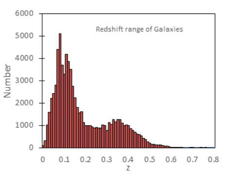
The photometric catalog dataset used in this study was originally sourced from SDSS DR 13, covering 150,000 galaxy samples. In order to ensure the high quality of the built model, this article selects the low amplitude error samples with average values less than 0.1 for training: g_ err、r_err、i_err and z_err. After screening, the remaining number of samples is 80218, with a red shift range from 0 to 0.8. The histogram of the sample redshift distribution is shown in Figure 1. The high-dimensional and nonlinear characteristics of photometric data give it unique complexity. In order to minimize the impact of sample differences, we divided galaxies into early type galaxies with a reddish color and late type galaxies with a bluish color, in order to improve the prediction accuracy of the model.
Introduction of AutoGluon-Mix and Related Comparative Algorithms
AutoGluon is an open source AutoML framework [9]. Unlike existing AutoML frameworks that mainly focus on model and hyperparameter selection, our research adopts a multi model fusion method in AutoGluon-Mix to leverage the advantages of model fusion and shorten training time. At the same time, we have also introduced some beneficial related technologies from deep networks to further improve the performance of AutoGluon-Mix.
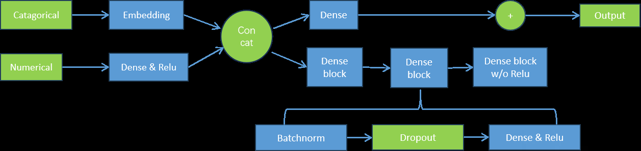
The network structure adopted by AutoGluon-Mix is shown in Figure 2 (feed forward neural network). In the figure, the layers with trainable parameters are marked in blue. The network will apply an independent embedding layer for each classification feature, and the dimension selection of the embedding layer is proportional to the number of unique levels contained in that feature. DenseNet uses Concat connection method, which uses cross channel splicing to connect features at different levels. DenseNet is divided into multiple Dense Blocks, with consistent feature map sizes within each block. Different Dense Blocks are down sampled and connected through a Transition module. Relu is a linear rectification function commonly used in the activation function of neural networks, which turns negative values to zero while keeping positive values unchanged. BatchNorm is a technique for normalizing a batch of data in a training set. By normalizing each feature in a small batch of data, the training process of the network can be accelerated, and the stability and convergence speed of the model can be improved.
AutoGluon Mix introduces an innovative integrated stacking method, as shown in (Figure 3). This method uses two stacked layers and combines n basic models.
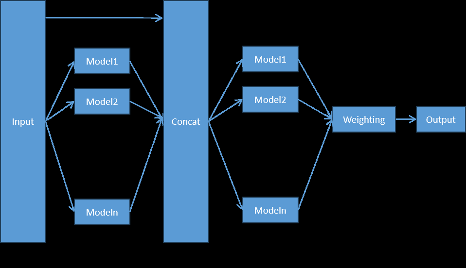
Base Layer
Contains n basic models whose outputs are connected and then passed on to the next layer. The stacked layer model takes the predicted results of the previous layer model and the original data features themselves as inputs.
Stack
In the stack layer, the same basic model as the base layer (with consistent hyperparameters) is used as the stacker.
Output Layer
By combining multiple stacked layers with weights, the final prediction result is obtained.
AutoGluon-Mix also introduced K-fold bagging technology to help reduce the variance of prediction results. The implementation of K-folding bagging is to randomly divide the data into k disjoint blocks, and then use different data blocks retained in each copy to train the model of k copies. AutoGluon Mix has packaged multiple models, including K Nearest Neighbors, Random Forests, XGBoosted trees, LightGBM boosted trees, CatBoost boosted trees, Extremely Randomized Trees, and neural networks. During the training process, each model needs to generate out of fold (OOF) predictions for data blocks that it did not use during the training period.
This study compares several different algorithms, including traditional BP neural network, ensemble algorithm XGBoost, combination algorithm PSOBP, and FOABP- RF. Compared with traditional GBDT, XGBoost has made some technological improvements, which have resulted in significant performance improvements in supervised learning applications. The PSOBP algorithm is an algorithm that utilizes Particle Swarm Optimization (PSO) to optimize BP neural networks. This method combines the PSO algorithm with the BP neural network to achieve better performance and convergence when optimizing the parameters and weights of the neural network. The FOABP-RF algorithm is a combination of Fruit Fly Optimization Algorithm (FOA), BP neural network, and Random Forest (RF). Research has shown that in the field of redshift photometry, the FOABP- RF algorithm performs better than using a single algorithm alone. The advantage of this combination algorithm is that it can fully utilize the characteristics of different algorithms, thereby improving overall performance.
Results and Analysis
Feature Selection
The data is divided into training and testing sets in a 6:4
ratio. The initial input consists of 15 features, consisting of photometric values from the five bands u, g, r, i, and z, as well as the differences in color features between the low and high bands. Then, an additional error values of these five bands ,u_ err, g_ err, r_ err, i_ err, z_err, was added, which totaling 20 features, are used as inputs for the model. The output of the model is the prediction of the photometric redshift value, as shown in Table 1.
| Feature | f1 | f2 | f3 | f4 | f5 | f6 | f7 | f8 | f9 | f10 |
|---|---|---|---|---|---|---|---|---|---|---|
| Input physical value | u | g | r | i | z | u-g | u-r | u-i | u-z | g-r |
| Feature | f11 | f12 | f13 | f14 | f15 | f16 | f17 | f18 | f19 | f20 |
| Input physical value | g-i | g-z | r-i | r-z | i-z | u_err | g_err | r_err | i_err | z_err |
Table 1: Correspondence between Feature and Input Physical Value.
Table 2 compares the mean square error of different algorithms using only 15 features and 20 features for early type galaxies. From the table, it can be seen that various algorithms significantly reduce the mean square error after adding these additional 5 features. This indicates that these five features,u_err,g_err,r_err,i_err,z_err,are closely related to redshift.
| Input | AutoGluon-Mix early | XGBoost | BP | CNN | PSOBP | FOABP-RF early |
|---|---|---|---|---|---|---|
| early | early | early | early | |||
| Feature (20) | 0.00121 | 0.00143 | 0.0015 | 0.0016 | 0.0014 | 0.00138 |
| Feature (20) | 0.00157 | 0.00162 | 0.0017 | 0.0017 | 0.0017 | 0.00164 |
Table 2: Mean Error of Different Algorithms (using 15 And 20 Eigenvalues respectively).
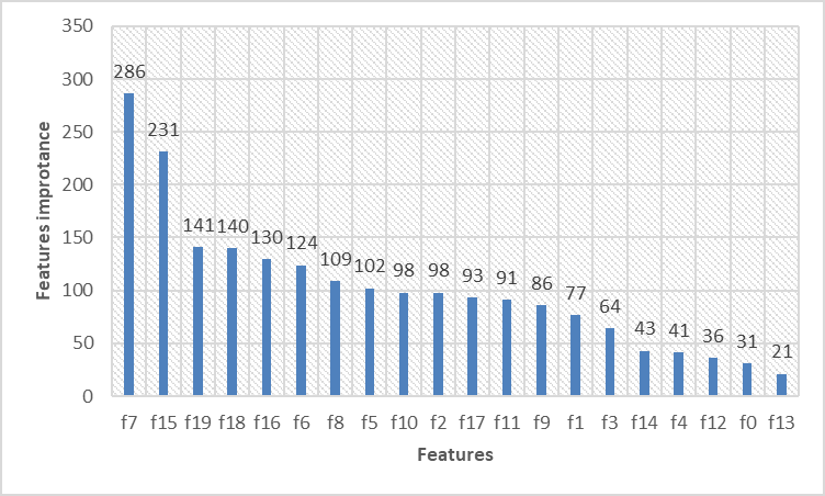
In Figure 4, we demonstrate the importance score of input features. F15 to f19 represent the five newly added features u_ err, g_err, r_ err, i_err, z_err. The larger the value, the higher the importance of the feature. Moreover, 4 of these 5 new features have entered the top 5, indicating that their addition has significant implications for improving the accuracy of galaxy redshift estimation. This confirms that these adding new features is essential for improving estimation performance.
Evaluation Indicators
In machine learning tasks, it is a crucial stage that to determine appropriate evaluation indicators to measure the performance of the model. For regression tasks such as redshift estimation, we focus on evaluating the difference between predicted and actual values. The commonly used indicators for regression model evaluation include: mean square error (MSE), root mean square error (RMSE), deviation ∆ 𝑍, mean Bias of ∆ 𝑍, normalized median absolute deviation (NAMD) of ∆ 𝑍, Outliers, etc. 3.3 Experimental results The experimental results of AutoGluon-Mix and other comparative algorithms have been summarized in Table 3. Due to the correlation between evaluation indicators and errors, a smaller value indicates better algorithm performance. In each row of the table, the best results are annotated in bold font. In terms of Bias metrics, the results show that the XGBoost algorithm performs more stably. In terms of Outliers indicator, the results of the PSOBP algorithm indicate that it has the least number of Outliers. However, in terms of the other 4 indicators MSE, RMSE, ∆ 𝑍, and NMAD, AutoGluon-Mix performed the best. By combining multiple indicators, it can be concluded that AutoGluon Mix has high quality results, and this algorithm has advantages in accuracy, bias, and result stability. In the study of early type galaxies, compared to algorithms such as BP, CNN, FOABP-RF, PSOBP, and XGBoost, the MSE of AutoGluon Mix was reduced by 16.55%, 23.42%, 12.32%, 14.79%, and 15.38%, respectively. In the study of late galaxies, the MSE of AutoGluon Mix was reduced by 14.29%, 21.05%, 14.69%, 21.40%, and 11.33%, respectively, compared to algorithms such as BP, CNN, FOABP-RF, PSOBP, and XGBoost.
| Indications | AutoGluon-Mix early | XGBoost | BP | CNN | PSOBP | FOABP-RF early |
|---|---|---|---|---|---|---|
| early | early | early | early | |||
| MSE | 0.00121 | 0.00143 | 0.0015 | 0.0016 | 0.00142 | 0.00138 |
| RMSE | 0.03842 | 0.03781 | 0.0381 | 0.0398 | 0.03777 | 0.03723 |
| △Z | 0.02766 | 0.02978 | 0.0305 | 0.0317 | 0.03013 | 0.02953 |
| Bias | 0.00041 | 0.0001 | 0.0011 | 0.0013 | 0.00077 | 0.00054 |
| NMAD | 0.02089 | 0.02224 | 0.024 | 0.0241 | 0.02307 | 0.02154 |
| Outliers | 0.01278 | 0.01287 | 0.013 | 0.0137 | 0.01283 | 0.01366 |
| Indications | AutoGluon-Mix late | XGBoost | BP | CNN | PSOBP | FOABP-RF late |
| late | late | late | late | |||
| MSE | 0.0018 | 0.00203 | 0.0021 | 0.0023 | 0.00229 | 0.00211 |
| RMSE | 0.0425 | 0.0451 | 0.0459 | 0.0487 | 0.04784 | 0.04599 |
| △Z | 0.03321 | 0.03529 | 0.0364 | 0.0376 | 0.03801 | 0.03593 |
| Bias | 0.00135 | 0.0006 | 0.0018 | 0.0041 | 0.00243 | 0.00104 |
| NMAD | 0.02442 | 0.02535 | 0.0281 | 0.0289 | 0.02751 | 0.02549 |
| Outliers | 0.01404 | 0.01618 | 0.0152 | 0.015 | 0.0129 | 0.01597 |
Table 3: Experimental Results of Autogluon Mix and other Comparative Algorithms.
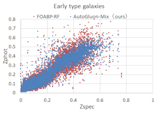
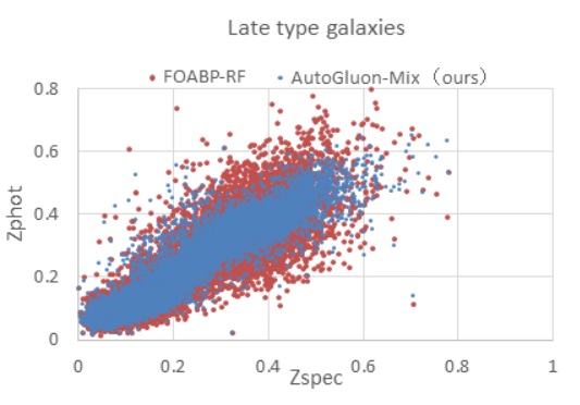
In Figure 5, we present a scatter plot using AutoGluon- Mix and FOABP-RF for redshift estimation of early and late galaxies. ‘Zspec’ represents spectral redshift, and ‘Zphoto’ represents estimated redshift. In the figure, the blue dots represent the estimation results of AutoGluon Mix, and the red dots represent the estimation results of the FOABP- RF algorithm. From the figure, it can be observed that the estimation results of the two algorithms are generally similar, showing a diagonal trend from the bottom left corner to the top right corner. However, the results estimated by AutoGluon-Mix are more concentrated and closer to the true values. This also indicates that AutoGluon-Mix is superior in the estimation performance.
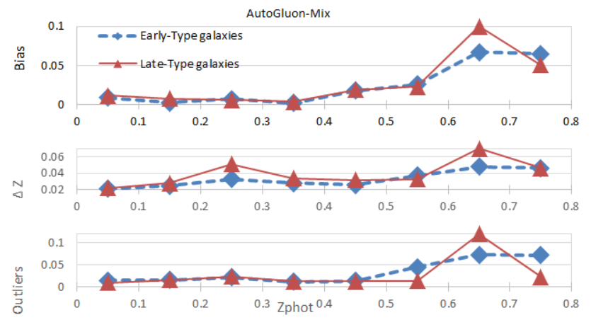
In Figure 6, the relationship diagrams are drawn between the 3 indicators of Bias, ΔZ, Outliers and the estimated redshift. The values of the 3 indicators are all less than 0.1.
Overall, the estimation performance of the AutoGluon-Mix is quite good, especially when the estimated redshift is less than 0.6, the values of the 3 indicators remains very low.
Conclusion
This study proposes a novel ensemble algorithm, AutoGluon-Mix, for estimating galaxy redshift from photometric catalog data. The multi-layer stacking integration method adopted by AutoGluon-Mix integrates the advantages of multiple basic models, significantly improving the accuracy of estimation; meanwhile, the introduction of K-fold bagging helps to reduce the risk of overfitting. By analyzing the importance of features, it can be found that the errors in the 5 bands u, g, r, i, and z play an important role in estimating galaxy redshift. Therefore, we have introduced these 5 additional features as inputs to the network. The AutoGluon Mix algorithm is compared with 5 algorithms, including BP, PSOBP, CNN, FOABP-RF, and XGBoost, in multiple aspects, and is visually analyzed the experimental results. The performance of the AutoGluon-Mix is evaluated from a detailed perspective by drawing multiple correlation functions in different redshift intervals.
All results have proven that AutoGluon-Mix performs best among numerous algorithms. In early galaxies, compared to the algorithms such as BP, CNN, FOABP- RF, PSOBP, and XGBoost, the MSE of the AutoGluon Mix algorithm decreased by 16.55%, 23.42%, 12.32%, 14.79%, and 15.38%, respectively. In late type galaxies, compared to algorithms such as BP, CNN, FOABP-RF, PSOBP, and XGBoost, the MSE of the AutoGluon Mix algorithm has been reduced by 14.29%, 21.05%, 14.69%, 21.40%, and 11.33%, respectively.
References
-
Salvato M, Ilbert O, Hoyle B (2019) The many flavours of photometric redshifts. Nature Astronomy 3(3): 212-222.
-
Lima EVR, Sodre L, Bom CR, Nakazono L, Teixeira GSM, et al. (2022) Photometric redshifts for the S-PLUS Survey: Is machine learning up to the task?. Astronomy and Computing 38: 2110.13901v2.
-
Jingchang P, Ali L, Peng W, Jiang B, Yin-bi L, et al. (2016) A method for measuring the spectral redshift of low- quality galaxies based on multi resolution fusion distance. Spectroscopy and Spectral Analysis 36(5): 1521-1525.
-
Sisodiya N, Dube N, Prakash O, Priyank T (2023) Scalable big earth observation data mining algorithms: a review. Earth Science Informatics 16(3): 1993-2016.
-
Zhou H, Che A, Shuai X, Yi Z (2023) A spatial evaluation method for earthquake disaster using optimized BP neural network model. Geomatics, Natural Hazards and Risk 14(1): 1-26.
-
Wang Y, Zhang Y, Dong Z (2022) Neural Network-Based Approach for Evaluating College English Teaching Methodology[J]. Mathematical Problems in Engineering pp: 1-8.
-
Ziemba P, Becker J, Becker A, Aleksandra IRZ, Mateusz P, et al.(2021)Credit Decision Support Based on Real Set of Cash Loans Using Integrated Machine Learning Algorithms. Electronics 10(17): 2099.
-
Ravindran SM, Bhaskaran SKM, Ambat SK, Kannan B, Manoj MG (2022) An automated machine learning methodology for the improved prediction of reference evapotranspiration using minimal input parameters. Hydrological processes 36(5): e14571.
-
Jiang CS, Li YD, Wang ZD (2012) A Study on Optimization of Automotive Suspension Base on PSO-BP Network Algorithm. Applied Mechanics & Materials 121-126: 3760-3764.
- Asymmetry Irreversible Heterogeneity Quantum Cosmology Grand Mathematical PHYSICS
- Early Universe: Hadronic Crystals Coherent Micro Gravitational Wave Emitters PHYSICS Part II
- The Solar System Constraint Maze: A Scientific Dead-End Revealing the Interuniversal Machine
- Assessment of Radiofrequency Radiation from 2G and 3G Mobile Phone Handsets
- Early Universe Magneto-Gravitational Coupling Genesis Physics: Part I
- Falsifiability of the Classical Law of Gravitation and Unveiling the Time-temperature Entanglement of the Universe