Technical Efficiency of Smallholder Farmers Wheat Production: The Case of Debra Libanos District, Oromia National Regional State, Ethiopia
This study aimed to examine the technical efficiency of smallholder farmers in wheat production in the Debra Libanos district. Two stages sampling technique was used to select 150 sample farmers to collect primary data using crosssectional data of 2018/19 production season. Data analysis was carried out using descriptive statistics like mean, minimum, maximum, frequency and standard deviation and econometric models such as stochastic production frontier and two-limit Tobit regression models to estimate level and identify factors affecting technical efficiency respectively. The estimated stochastic production frontier model indicated that land, labor, seed and chemical fertilizer were positively and significantly affects farmers’ wheat production level. The study indicated that the average technical efficiency level of wheat producing farmers was 78.5% implying that there was technical efficiency variation among smallholder farmers in the study area. In other words, the average wheat yield loss due to technical efficiency variation was 5.13 qt per ha. Therefore, these results implied that there is a room to increase the efficiency of wheat production in study area. Moreover, the two-limit Tobit regression model results showed that age, family size, livestock size, frequency of extension contact and frequency of ploughing had positive and significant effect on technical efficiency. Hence, attention should be given to improve the efficiency level of those less efficient farmers by adopting the practices of relatively efficient farmers in the study area. Besides this, policies and strategies of the government should be directed towards the above mentioned determinants.
Introduction
In developing countries agricultural production often falls short of its potential. In sub-Saharan Africa, the majority of agricultural producers are comparatively poor, smallholder farmers with limited use of fundamental technologies such as sufficient seeds and fertilizers [1]. Ethiopian economy dominated by agriculture, in terms of its contribution to Gross Domestic Product (GDP), employment opportunities, foreign exchange earnings, income and food source. It accounts for about 35.8% of the GDP, provides employment to more than 83% of total population that is directly or indirectly engaged in agriculture, generates about 79% of the foreign exchange earnings of the country and raw materials for 70% of the industries in the country [2]. In Ethiopia, about 1.7 million hectare (ha) wheat was cultivated by about 4.2 million smallholder farmers. The average wheat yield was about 27.4 qt per ha, during 2017/18 cropping season [3]. In Oromia, Amhara and SNNP, the wheat area coverage from cereal crops was 19%, 16% and 14% and the productivity of wheat was 29.7, 25.3 and 26.7qt per ha respectively. And Oromia region accounts for 53% of the total area and 58% of production from the national level wheat production. From the total area of cereal crops in the North Shoa zone, wheat accounts for 21% and in terms of production, it accounts for 24%. Additionally, in the zone 52% of farmers were wheat producer and a productivity of wheat was 25 qt per ha [3]. According to the Debra libanos district agricultural office (DLDAO) annual crop assessment year of 2018/19, from the total area crops cultivated, wheat accounts for 38% and the productivity was 21 qt per ha. Even though, the district has higher potential from cereal crops next to teff, productivity of wheat was low, which was less than the productivity of the country, region and zone. As observed from the study the minimum output of wheat was 6.5 qt per ha while the maximum output was 38.5 qt per ha. So, there was disparity of productivity between wheat producers in the district due to difference in input application rates and management practices. Hence, understanding the level and determinant of technical efficiency variation among wheat producers might support to assess the opportunities for increasing wheat production and productivity. Therefore, this study was designed to analyze technical efficiency of smallholder farmers in wheat production in the Debra Libanos district, North Shoa zone, Oromia national regional state, Ethiopia.
Statement of the Problem
The agriculture sector in Ethiopia plays important roles in food security, economic growth, foreign exchange earnings, poverty alleviation and employment creation. Despite the many contribution over the past years, its importance is inadequate because of different factors such as low level of crop management practices and lack of improved production technologies. Therefore it is difficult to meet the food requirements of the growing population [4, 5]. In addition, in areas where there is technical efficiency variation, introduce new technology may not bring the expected impact, unless factors associated with efficiency variation among farmers are identified and acted upon. And also use either the introduction of current agricultural technologies or improving the efficiency of farmers [6]. The productivity of wheat as world was 33.2 qt per ha [7]. In Ethiopia, wheat is the most widely grown and planted cereals by farmers. Whereas, farmers in the Debra Libanos district are practice mixed farming. But, crop production is the dominant component of the farming system. Among the cereals grown, teff and wheat are the major crops both in terms of area cultivated and volume of production. According to the DLDAO (Debra Libanos District Agricultural office) annual crop assessment production season reports, from the total area of crop cultivated wheat accounts for 4,178 ha and its productivity was 21qt per ha in the study area. However, the productivity was less by 8.7 qt per ha from regional wheat average productivity and 4 qt per ha from zone wheat average productivity. Thus, this study was used to explore the problem related to the efficient use of resources in the study area. In other way, different studies indicated that a number of factors can affect the technical efficiency level of farmers, but those factors are not equally important and similar in all places at all time. Therefore, strategy implications drawn from some of the empirical works may not allow in designing area specific policies to be compatible with its socio-economic as well as agro ecologic conditions and the results of some of the studies may not allow making a comparative analysis of farmer's technical efficiency across kebeles. So, it is important to fill this noticeable knowledge gap by studying technical efficiency of wheat and get current information. Finally, many empirical studies did not consider yield gaps due to technical efficiency variation among wheat producers and money value (birr) of the lost yield, which is very important for policy and decision makers. Thus, this study attempted to determine the amount of wheat lost due to technical efficiency variation in the study area. So, researcher was initiated to conduct on this issue to get recent scientific result and bridge the current information gap by providing empirical evidence on smallholder farmers’ resource use efficiency by using cross-sectional data that was collected from randomly selected sample farmers who were involved during 2018/19 production season in the district.
Research Methodology
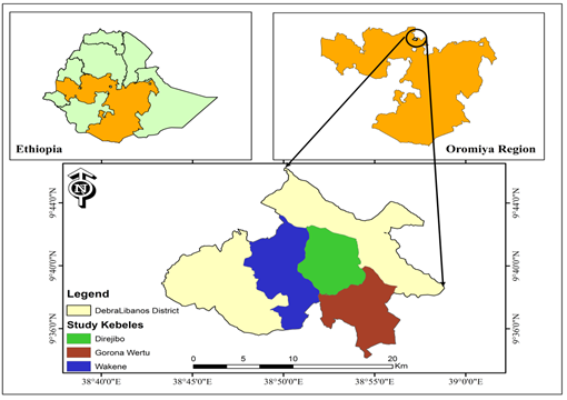
Description of the study area: The study is carried out in Debra Libanos district, North Shoa zone, Oromia national regional state, Ethiopia. It is located between 380 40’ 0” E and 390 0’ 0” E longitude and 90 36’ 0’’N and 90 40’ 0’’N latitude with altitude ranging from 1500 to 2700m above sea level (Figure 1). The district capital town, Shararo, is about 89 km away from Addis Ababa. The district has 10 rural and 1urban kebeles. A total population of this district is 49346, of whom 25501 (52%) are men and 23845 (48%) are women. From the total population, the rural dwellers are 39210 (79%) and urban dwellers are 10136 (21%) [8].The district has a total area of 29776 km2. With regard to land use pattern of the district, cultivable land 70% and the agro-climatic feature of the district is tropical as 75%, 15% and 10% are highland, midland and lowland respectively. The major soil types in the district are clay soil 63%, mixed soil 27% and sandy soil 10%. Debra Libanos is characterized by medium rainfall with a mean annual rainfall of 1000 mm that ranges from 800-1200 mm. The annual temperature is from 150C-230C. The total cultivated land and number of farmers in the district is 20818 ha and 5868 respectively. From the total number of farmers, 5222 (89%) are males and 646 (11%) are females. The main staple food crops grown around the study area are teff, wheat, maize, sorghum, bean, chicken pea and horticultural crops such as onion and carrot. Livestock production is also one of the major economic bases in the district. Community pasture and straw from crops are the main sources of feed for livestock production. Types of livestock in the studied area are cattle (60120), sheep (47718), goats (5989), horses (7160), donkeys (12757), mules (234) and poultry (36870) [9].
implementation of the actual survey for its validity and content, and to make overall improvement of the same and in line with the objectives of the study. In addition, secondary data was gathered from DLDAO, CSA (central statistical agency), published articles and unpublished documents. Sampling technique and sample size determination: Two-stage sampling techniques were employed to select sample farmers. In the first stage, 3 kebeles are selected randomly from 7 wheat producers’ kebeles. In the second stage, 150 sample farmers were selected using simple random sampling technique based on probability proportional to the size of wheat producers in the 3 selected kebeles. The sample size is determined based on [10] formula. The simplified formula to calculate the sample size was:- 𝑛= N 1 + N(e)2 Where: n =sample size, N = total number of wheat producers in study area, e = level of precision which is 8% (since, the producers have homogeneity characteristics) and 1 is for designates probability of the event occurring. Yamane’s formula was used because of its homogenous type of population in the study area and known population and 8% of precision level was applied for the purpose of managing all samples in terms of the available resource that the researchers have including cost, time, etc.
| Name of Kebeles | Total wheat producing farmers | Sample farmers | ||||||
|---|---|---|---|---|---|---|---|---|
| Goro Wertu | 803 | 58 | ||||||
| Wakene | 745 | 53 | ||||||
| Dire Jibbo | 542 | 39 | ||||||
| Total | 2090 | 150 |
Table 1: Sample farmers of three kebeles. **Method of data analysis:** To address the objectives of this research, two types o
Source: Own computation based on the district data (2019) Table 1: Sample farmers of three kebeles. Method of data analysis: To address the objectives of this research, two types of analysis, namely descriptive and econometric analyses were used for analyzing the collected data. In addition, Stata version 14 software program was used to analysis the data. Descriptive Analysis: Descriptive statistics such as mean, maximum, minimum, standard deviation, frequency and percentage of variables were computed to characterize the socio-economic, demographic, institutional, farm characteristics and the distributions of technical efficiency levels of the sampled farmers in the study area. Econometric analysis: In the study area, wheat is rain- fed crops which may be affected by random shocks such as drought and irregular rainfall. The farmer may deviate from the frontier not only because of measurement error, statistical noise or any other influence but also because of technical efficiency variation. To assess such conditions the stochastic frontier model was used in the analysis of technical efficiency of wheat production in the study area. Thus, a stochastic frontier model is preferred because of its capable of capturing measurement error and other statistical noise influencing the shape and position of the production frontier. A stochastic production frontier (SPF) model proposed by the accordance with the original models are applied to cross-sectional data to determine the technical efficiency [11]. Hence, most recent studies on technical efficiencies found in agriculture have used the stochastic frontier model to account for random noise [12, 13, 14, 15, 16]. The general SPF model is specified as.
ym = f(Xm; β) + εm m=1, 2, 3,..., k, where 𝑦𝑚the production of the mth sample farmer, 𝑓(𝑋𝑚;β) was the convenient frontier production function (e.g. Cobb-Douglas or Translog), 𝑋𝑚 is a vector of inputs used by the mth sample farmer, β is a vector of unknown parameters, 𝜀𝑚 is a composed disturbance term made up of two error elements ( v𝑚and u𝑚) and k represents the number of farmers who was involved in the survey.
Among the production function, Cobb-Douglas and translog production functions had been the most popularly used models in the most empirical studies of agricultural production analysis. Some researcher argues that Cobb-Douglas functional form had advantages over the other functional forms in that it provides a comparison between the adequate fit of the data and computational feasibility. It was also convenient in interpreting elasticity of production and it was very parsimonious with respect to degrees of freedom. According to [17], the Cobb-Douglas functional form had the most attractive feature which was its simplicity.
A logarithmic transformation provides a model which is linear in the logs of inputs and hence it lends itself to econometric estimation. But, the translog production function was more complicated to estimate having serious estimation problems. One of the estimation problems was as the number of variable inputs increases, the number of parameters to be estimated increases rapidly. In addition, the additional terms require cross products of input variables, thus making serious multicollinearity and degrees of freedom problems.
Cobb-Douglas model assumes unitary elasticity of substitution, constant production elasticity and constant factor demand, if the interest was to analyze the efficiency measurement and not analyzing the general structure of production function, it had adequate representation of technology and insignificant impact on the measurement of efficiency [18]. When farmers operate in small farms, the technology was unlikely to be substantially affected by variable returns to scale [17]. Moreover, Cobb-Douglas production function had been employed in many types of research dealing with efficiency [14, 15, 16, 19, 20, 21, 22, 23]. So, it was adopted for this study. Thus, Cobb-Douglas frontier function was specified as follows:
β2 … Xn
β1X2 βn The linear form of Cobb-Douglas production function for this study was defined as:
Ym = AX1
5 ln(Ym) = β0+ ∑βnlnXmn + εm n=1 ln (Ym) = β0 + β1ln SEED + β2lnLND +β3lnLAB
+ β4lnCHEMFER + β5lnOXEN + εm εm = vm −um Where, ln denotes the natural logarithm, n was represents the number of inputs used, m represents the mth farmer in the sample, ym represents the observed wheat production of the mth farmer, Xmn denotes nth farmer input variables was used in wheat production of the mth farmer, β0 represents intercept, β1 −β5 stands for the vector of unknown parameters would be estimated and elasticity of production , εm a composed disturbance term makes up of two elements (vm and um), vm accounts for the stochastic effects beyond the farmer’s control, measurement errors and other statistical noises and, um captures the technical efficiency variation. Then the TE scores of the given farmer was calculated as followed:
Y∗= = f(Xm, β)(expVm−Um)
TEm = Ym
f(Xm, β)(expVm) = exp(−um) Where, Y∗ = frontier output, Ym = actual output In this study technical efficiency estimated from SPF regressed by using a censored two-limit Tobit regression model on farm-specific independent variables that explained efficiency variation across wheat producers. The rationale behind using a two-limit Tobit regression model was that there were a number of farm units for which efficiency was bounded in nature between 0 and 1. That was the distribution of efficiency was censored above from unity and below zero. The use of the Tobit model was intuitive because the parameter estimates were biased and inconsistent if OLS was used (Gujarati, 2004). This is because OLS underestimated the true effect of the parameters by reduced the slope (Goetz, 1995). The degree of bias would also increase as the number of observations that take on the value of zero increases. This suggests that OLS regression was not appropriate and estimation with OLS would have led to biased parameters estimates. Therefore, the two-limit Tobit regression model offered the most preferred option and specified as follows:
12 + um ∗ = δ0 + ∑δLXmL
Em ,TE
L=1
Where, m referred to the mth farm in the sample farmers; L was the number of factors affecting (technical efficiency) TE; Em was technical efficiency scores representing the (technical efficiency) TE of the mth farm. Em ∗ was the latent variable, δ0 was intercept, δL were unknown parameters would be estimated, um was a random error term that was independently and normally distributed with mean zero and common variance and XmL were demographic, institutional, socio-economic and farm-related variables which were expected to affect technical efficiency. Denoting Em as the observed variables, ∗≥1 Em
1 if Em
]
∗ if 0 < Em
∗< 1 0 if Em
Em = [
∗≤0
Results and Discussion
Result of Descriptive Analysis
| Family Size: | The average family size of the sampled | |
|---|---|---|
| farmer was 5.9 with the minimum 1 and maximum 9. The | ||
| result implies that the average family size in the study | ||
| area was higher than the national average family size | ||
| which is about 5.2 persons per farmer [23]. So, large | ||
| family size is a source of labor for farming practice in | ||
| developing country like Ethiopia especially in the study | ||
| area. |
Table 2: Age, educational level, family size and livestock size of sample farmer. Sex: About 84% of the sample farmers were male
Livestock size: Given a mixed farming system in the study area, livestock has a great role as a source of income. And also, farmers who have more livestock holding may not have difficulties to purchase inputs of production like seed and fertilizer. The type of livestock kept by sampled farmers includes cow, oxen, horse, donkey, calf, sheep, heifer and hen. Among others, oxen power is the major input in crop production process serving as a source of draught power. The mean of the livestock holding of the sampled farmers in the study area was 13.33 TLU per sample farmer. This implies that most of the sample farmers have enough livestock to involve in wheat production practice such as for timely land preparation, sowing, harvesting, transportation and threshing. Education: It is a tool to modernize farming systems through the adoption of new technologies and practices. In addition to this, it would help farmers to able to produce higher output using the existing recourses more efficiently through increasing their information acquisition and decision making abilities. The average educational level of the sample farmers during the survey period was about 6.6 years with the minimum 0 and maximum of 12 years of schooling (Table 2)
| Variables | Min | Max | Mean | Std. Dev. | ||||||||||
|---|---|---|---|---|---|---|---|---|---|---|---|---|---|---|
| Age | 22.00 | 48.00 | 40.26 | 5.92 | ||||||||||
| The educational level | 0.00 | 12.00 | 6.57 | 3.69 | ||||||||||
| Total number of families | 1.00 | 9.00 | 5.59 | 2.49 | ||||||||||
| Total number of livestock | 2.00 | 25.00 | 13.33 | 5.39 |
Table 3: Age, educational level, family size and livestock size of sample farmer. Sex: About 84% of the sample farmers were male
Table 2: Age, educational level, family size and livestock size of sample farmer. Sex: About 84% of the sample farmers were male headed and the remaining 16% were female headed. It was understood that female headed farmers face greater challenges in agricultural production and marketing compared with their male headed counterparts. This is due to the fact that females are the one who is responsible for the many farmer domestic activities and may not accomplish the farming activities on time. Off/non-farm activities: -The livelihood of farmers also relies on different off/non-farm activities during the production season in addition to the farm activities. From total sample farmers, (105)70% of them have reported that they were involved in off/non-farm activities such as carpenter, wage, tailors, weaving and selling of firewood. However, (45)30% of the total sample farmers were busy in agricultural activities (not involved in off/non-farm activities. Farm Size: Farmers use most of their land for crop production and grazing. The average farm size of the sampled farmer was 1.8 ha. Out of total, on average, 76% of the land (1.37 ha) is cultivated. The result implies that 76% sample farmers have relatively larger farm size compared to that of the national average of farmers in Ethiopia which is 1.2 ha (Essa, 2011) and the holdings of the remaining 24% of the farmers are less than 1.2 ha. The mean land size allocated for wheat production was 0.76 ha and its standard deviation was 0.40.
The Distance of Home From The Nearest Market: The survey result showed that, the average walking distance of the nearest market from the farmer's home was 42.77 minutes. Frequency of Extension Contact: Extension services usually play a major role in disseminating new and improved farming techniques. The major sources of agricultural information for farmers are extension agents. Regular contact with extension agents makes farmers be aware of the adoption of new technologies which helps them to maximize agricultural production and productivity. The extension agents contact farmers on different intervals; some farmers are being contacted more frequently while others have got less chance at all to be contacted by extension agents. Accordingly, the survey result, sample farmers were being contacted by extension agents on average 4.83 times with the minimum of 1 time and maximum of 6 times during 2018/19 production season in the study area. Frequency of Ploughing: The number of ploughing indicates an intensity of land preparation that helps for appropriate germination of the seed which is expected to have a direct impact on yield. Sample farmers were ploughing their wheat farm average 4.25 times with a minimum of 2 times and a maximum of 5 times.
| Variables | Min | Max | Mean | Std. Dev. | |||||||
|---|---|---|---|---|---|---|---|---|---|---|---|
| Farm size (ha) | 0.00 | 5.50 | 1.37 | 1.01 | |||||||
| Extension contact | 1.00 | 6.00 | 4.83 | 1.49 | |||||||
| Frequency of ploughing | 2.00 | 5.00 | 4.25 | 0.96 | |||||||
| Distance of farmer home | 10.00 | 120.00 | 42.77 | 25.24 | |||||||
| Frequency of weeding | 0.00 | 4.00 | 1.25 | 0.63 |
Table 4: Farm size, extension contact, frequency of ploughing and distance from market.
Source: Own computation (2019) Table 3: Farm size, extension contact, frequency of ploughing and distance from market.
| Types of crops | Area coverage(ha) | Production(qt) | |||||||||||
|---|---|---|---|---|---|---|---|---|---|---|---|---|---|
| Mean | Std. Dev. | Mean | Std. Dev. | ||||||||||
| Teff | 1.09 | 0.64 | 8.15 | 6.16 | |||||||||
| Wheat | 0.76 | 0.40 | 15.30 | 10.89 | |||||||||
| Barley | 0.05 | 0.10 | 0.37 | 0.89 | |||||||||
| Bean | 0.46 | 0.32 | 3.39 | 2.82 | |||||||||
| Chickpea | 0.13 | 0.22 | 1.08 | 2.39 |
Table 5: Area coverage, production and productivity of major crops of sample farmer's. **Problems of wheat production:** The s
Source: Own computation (2019) Table 4: Area coverage, production and productivity of major crops of sample farmer's. Problems of wheat production: The sample farmers mentioned that disease, high price of improved seed, weeds, high price of pesticides and shortage of rainfall were the problems they have been facing. The survey result indicated that about 68.67% of sample farmer respond that rust was the main problem affecting wheat production (Table 5). Types of problem Freq. Percent. Weeds 8 5.33 Low fertility of soil 4 2.67 Disease(Rust of wheat) 103 68.67 High price of improved seed 16 10.67 Shortage of rain fall 5 3.33 High price of pesticides 7 4.67
- Source: Own computation (2019)
- Table 5: Major problems of wheat production.
Table 6: Major problems of wheat production.
Description of variable used in production function: The average wheat output produced in the study area was about 15.3qt with a standard deviation of 10.9 among the sample farmers in 2018/19 production season which indicates the large difference of output among the farmers. The average land holding allocated to wheat production was about 0.76 ha with a standard deviation of 0.39 and ranges from 0.1875 to 3 ha. The average land allocated to wheat conforms to the fact that the farmers are small scale and held family managed and operated farm plots in the study area. On average 36.74 man equivalent labors were applied for wheat production with a standard deviation of 15.99. This shows that production existing among sample farmer was labour intensive. The average oxen labour used were 5.95 pair oxen. Ownership of oxen affects land preparation and management. Farmers who own more oxen use more labour and oxen draft power per ha, suggesting that oxen and labour are complements. Greater oxen ownership also increases the use of ploughing activities. On other hand, the average chemical fertilizer used was 1.41 qt. But the recommended rate of fertilizer is 2 qt per ha as the expert described. This implies that farmers used fertilizers below the recommended rate. In addition, the average seed rate used by the farmers in the study area was 1qt. But the recommended seed rates in the extension packages are between 1.25 to 1.75 qt per ha. This show that, the amount of wheat seed that sample farmers used was less than the amount recommended by the extension department.
| Variables | Mean | Std. dev. | Min | Max | ||||||||||
|---|---|---|---|---|---|---|---|---|---|---|---|---|---|---|
| Output(qt) | 15.300 | 10.886 | 3 | 95 | ||||||||||
| Total seed (qt) | 1.007 | 0.620 | 0.25 | 3.7 | ||||||||||
| Total land (ha) | 0.763 | 0.395 | 0.188 | 3 | ||||||||||
| Total labour (ME) | 36.741 | 15.986 | 2.4 | 84.3 | ||||||||||
| Fertilizers(qt) | 1.407 | 1.010 | 0.4 | 8 | ||||||||||
| Total oxen (pair oxen) | 5.947 | 3.0210 | 2 | 20 |
Table 7: Summary statistics of input variables used to estimate production function.
Source: Own computation (2019) Table 6: Summary statistics of input variables used to estimate production function.
Result of Econometrics Analysis
Hypothesis Test
Before going to analysis the parameter estimates of the production frontier and factors that affect the efficiency of the sample farmer's, the fittest function, model used and existence of efficiency variation were analyzed. Three hypothesis tests were applied using the generalized Likelihood Ratio (LR). The first hypothesis tested was, the test for the selection of the appropriate functional form for the data i.e. Cobb-Douglas versus Translog production function. The decision to select functional form depends on the calculated LR. Let the null hypothesis 𝐻0:𝛽nm = 0 is the Cobb- Douglas function and alternative hypothesis 𝐻1:𝛽mn ≠0 is the translog function. So, under the null hypothesis(𝐻0) the value of the LR function for the Cobb-Douglas production function is 5.5 while under the alternative hypothesis (𝐻1) for the translog function, the value of the LR function is 17.9.Then , 𝐿𝑅= −2(𝐻0 −H1) = −2(5.5 −17.9) = 24.8 . So, the calculated LR is equal to 24.8 and the critical value at 15 degree of freedom and 5% significance level is 25.0. This implies that the calculated LR is less than the critical value. Thus, the null hypothesis that all coefficients of the interaction terms in Cobb-Douglas specification are equal to zero was accepted. Hence, the Cobb-Douglas functional form was used to estimate the efficiency of the sample farmers in the study area.
The second hypothesis tested was, the test for the existence of the efficiency variation component of the composed error term of the stochastic frontier model. This is made in order to decide whether OLS best fits the data set as compared to the SPF. If the null hypothesis 𝐻0:𝛾= 0 is accepted against alternative hypothesis 𝐻1:𝛾≠0, then the spf is identical to OLS The third null hypothesis explored is that farm level efficiencies variation are not affected by the demographic, socio-economic, institutional and farm characteristics variables included in the efficiency determinant model i.e. 𝐻0:𝛿0 = 𝛿1 = ⋯𝛿12 = 0. To test this hypothesis LR is calculated using the value of the LR function under the Cobb-Douglas stochastic frontier model (model without independent variables of efficiency determinant model, 𝐻0 ) and the full frontier model (model with all independent variables of efficiency determinant model, 𝐻1). Under the null hypothesis(𝐻0) the value of LR function for a model without independent efficiency determinant variable is 5.5, while the alternative hypothesis (𝐻1) for the model with independent efficiency determinant variables, the value of the LR is 71.34. 𝐿𝑅= −2(5.5 −71.34) = 131.68 . The calculated LR value of 131.68 was greater than the critical value of ᵪ2 is 21.03 at 12 degree of freedom, this shows that the null hypothesis (𝐻0) that independent variables are simultaneously equal to zero was not accepted at 5% significance level. Hence, these variables simultaneously explain the sources of efficiency differences among the sample farmers.
Estimation of Production Function
The MLE of the parameters of the SPF specified were obtained using the Stata version 14 computer programs.
The result of the model showed that land, labor, chemical fertilizer and seed had a positive and significant effect on wheat production. Hence, the increase in these inputs would increase the production of wheat significantly as expected. The coefficients of the production function are interpreted as elasticity. The highest coefficient of output to land (0.37) indicated that land is the main determinant of wheat production in the study area.
| Variables | MLE | ||||||||||
|---|---|---|---|---|---|---|---|---|---|---|---|
| Parameters | Coefficient | Std. Err | |||||||||
| Constant | 𝛽 0 | 2.454*** | 0.302 | ||||||||
| LnSEED | 𝛽 1 | 0.270*** | 0.071 | ||||||||
| LnLND | 𝛽 2 | 0.390*** | 0.127 | ||||||||
| LnLAB | 𝛽 3 | 0.120** | 0.053 | ||||||||
| LnCHEMFER | 𝛽 4 | 0.305*** | 0.053 | ||||||||
| LnOXEN | 𝛽 5 | 0.062 | 0.120 | ||||||||
| Elasticity | 1.147 | ||||||||||
| Sigma square(σ2) | 0.128 | 0.022 | |||||||||
| Lambda(λ) | 2.488 | 0.057 | |||||||||
| Gamma(γ) | 0.861 | ||||||||||
| Likelihood | 5.5 |
Table 8: Estimates of the Cobb-Douglas frontier production function.
* and , significant at 1% and 5% level of significance, respectively. Source: Model result (2019) Table 7: Estimates of the Cobb-Douglas frontier production function.
𝜆2 (2.488)2 observed output can be derived 𝛾= (1+𝜆2) =
(1+(2.488)2) =
0.861. The estimated value of gamma (γ) was 0.861 which indicated that 86.1% of total variation in wheat output was due to technical efficiency variation.
Land allocated and chemical fertilizers are found to be statistically significant at a 1% significance level for wheat production, implies that increasing the level of these inputs would increase wheat production in the study area. Moreover, the coefficient for land use was 0.390, which implies that, at ceterius paribus, a 1% increase in the area of land allotted for wheat production, results in 0.390% increase in wheat output. Chemical fertilizers also appeared to be an important factor, with a coefficient of 0.305. This implies that a 1% increase in chemical fertilizers increase wheat output by about 0.305% at The returns to scale analysis can serve as a measure of total factor productivity [29] and the coefficients were calculated to be 1.147, indicating increasing returns to scale. This implies that there was potential for a wheat producer to continue to expand their production where resource use and production is believed to be inefficient. In other words, a 1% increase in all inputs proportionally would increase the total production by 1.147%. This result was consistent with [23] who estimated the returns to scale to be 1.266 in the study of efficiency of smallholder farmers in maize production in Oromia
national regional state, Ethiopia and 1.214 in the study of efficiency of wheat production West Shoa, Ethiopia respectively. But a study done by inefficiency sesame producers in Tigray [22], Ethiopia found returns to scale to be 0.926 which is decreasing returns to scale.
Efficiency Scores of Sample Farmers
In the Table 8 below the mean TE of sample farmers were 78.5%. Other studies support the finding. For example, [22] found mean TE of 71.4% for sesame producers in Tigray region; Ethiopia and [15] found mean TE of 79% for teff producers in Northern Shoa, Ethiopia. On average, if sample farmer in the study area operated at full TE level, they could increase their output by 17.8 % derived [(1 −
78.5
95.5) ∗100] from using the existing resources and level of technology. In other words, it implies that on average sample farmers in the study area can decrease their inputs (land, labor, oxen, chemical fertilizer and seed) by 17.8% to get the output they are currently getting. The most technically inefficient farmer would have an efficiency gain of 69.21% derived from [(1 −
29.4
95.5) ∗100] to attain the level of the most TE farmer.
| Types of efficiency | Mean | Std. Dev | . | Mi | n | Ma | x | |||||||
|---|---|---|---|---|---|---|---|---|---|---|---|---|---|---|
| TE | 78.5 | 0.117 | 29.4 | 95.5 |
Table 9: Yield gap analysis.
Analysis of Yield Gap in the Study Area
Productivity can change due to differences in the production technology, efficiency of the production process and environment in which production takes place. The yield gap always occurs due to TE variation among the farmers. So, analyzing of yield gap is an important system to estimate to what extent the production could be increased if all factors are controlled. It is computed as follows:
Ym Ym ∗.
𝑇𝐸m =
Then, solving for Ym
∗, the potential yield of each sample farmer was represented as:
∗= Ym
Ym
TEm
Where, TEm, the TE of the mth sample farmer in wheat production Ym
∗- the potential output of the mth sample farmer in wheat production in qt per ha and Ym- the actual output of the mth sample farmer in wheat production in qt per ha Therefore,yield gap (qt per ha) = Ym ∗−Ym
| Variables | Mean | Std. Dev. | Min | Max | |||||||||
|---|---|---|---|---|---|---|---|---|---|---|---|---|---|
| Actual qt per ha | 19.98 | 6.02 | 6.50 | 38.50 | |||||||||
| TE (%) | 78.5 | 0.12 | 29.4 | 95.5 | |||||||||
| Potential (qt per ha) | 25.12 | 5.22 | 16.21 | 42.17 | |||||||||
| Yield gap (qt per ha) | 5.13 | 2.58 | 1.25 | 15.40 | |||||||||
| Money lost (birr per ha) | 7183.69 | 3614.22 | 1750.05 | 21565.6 |
Table 10: Yield gap analysis.
Source: Own computation (2019) Table 9: Yield gap analysis.
In the table 9 above, it was observed that the mean wheat yield difference between sample farmer due to technical efficiency variation was 5.13 qt per ha. This implies that the sample farmers in were lost on average about 7,183.69 birr per ha estimated at (1qt = 1400.33birr).
Determinants of Technical Efficiency
The estimates of the two-limit Tobit regression model result also showed that among the twelve variables five (age, family size, livestock size, frequency of extension contact and plough) were found to be statistically significant in affecting the level of technical efficiency (Table 10). The results from the two-limit Tobit model were subjected to post estimation test using marginal effect analysis in order to estimate the trivial change from each factor that influences technical efficiency. Quantification of the marginal effects of these variables is a vital in order to estimate the change that will occur with respect to a change in one unit of that variable. Accordingly, the model results for each significant variable were discussed as follows:
Frequency of Extension Contact (EXTEN)
The coefficient for the frequency of extension contact had a statistically significant and positive relationship with TE at 1% significant level. This is consistent with the prior expectation that those farmers that had got more frequency of extension contact were more TE than those who with less frequency of extension contact with development workers. A positive effect of this variable suggested that farmers had more frequency of extension contact could lead them to improvements in resource allocation, facilitates the practical use of modern techniques, adoption of improved agricultural production practices and use inputs on the right way. The computed marginal effect result shows that, a unit increase in the number of extension contact would increase the probability of a farmer being technically efficient by 0.02% and the expected values of TE by about 2.18% and the overall efficiency of TE by about 2.21% a. This result was in line with the finding of [30, 23, 31].
Opposing to this, the studies found that extension contact negatively affects the efficiency due to extension workers are only concerned in increasing output and have not new skill and information to support the farmers [20, 14]. Specific to this study, the relative difference might be because of farmers who had high extension contact got new technology and correct management practices like timely sowing, weeding and can be used inputs as proper way. Age of the Sample Farmer's (AGE): Age of sample farmers had a positive and significant effect on TE of the wheat producer farmers in the study area at 5% significance level as expected. The results showed that younger farmer (productive age) with experience in farming leads to the gaining of better managerial skills over time, which made farmers able to allocate their resources more efficiently. The computed marginal effect result shows that a one year increase in the age of farmer's would increase the probability of a farmer being technically efficient by about 0.02% and the expected value of TE by 0.31% with an overall 0.31%. This is consistent with the findings of Kifle D, et al. [23]. Livestock size (LIVESZE): The result indicated that there was a positive and significant impact of livestock size on TE at 1% of significant level, which is corresponding with the expectation made as in the case of [14, 30, 31, 32] confirms the considerable contribution of livestock in reducing the current cost of inputs in wheat production. Given the importance of livestock in the crop production system as a source of draft power, food, income and inputs purchase. The model result seems logical to affect TE positively as expected. Moreover, a unit increase in the size of livestock (TLU) would increase
| Family size (FAMSZE): | The family size had positively |
|---|---|
| effect on TE of the wheat producer sample farmers at 5%, | |
| which was in line with expectation. Since the farmer with | |
| large number of family members might be able to use | |
| appropriate input combinations, due to the family is the | |
| main source of labour supply and it might be important in | |
| the production of wheat, as labour was a significant factor | |
| of production. The computed marginal effect result shows | |
| an increase the family size would increase the probability | |
| being of the farmer technically efficient by about 0.06% | |
| and the expected values of technically efficient by about | |
| 0.73% and with overall increases in the probability the | |
| level of TE by about 0.74%. Hence, the result was | |
| consistent with the found by | |
| [19,32-34]. |
Table 11: Tobit and marginal effect results of the TE determinants.
Frequency of Ploughing (FREQPLOU)
Frequency of ploughing had a positive effect on TE at 5% significant level as it was expected. Because timely and properly ploughing land used in order to make the soil compatible with crop growth. The computed marginal effect result shows that, a unit increase in the frequency of ploughing would increase the probability of a farmer being technically efficient by 0.18% and the expected values of TE by about 2.37% and the overall increase with the level of TE by about 2.39%. The result in line with [37] finding.
| Variables | Parameters | Tobit Result | Computed marginal effect | |||||||||||||
|---|---|---|---|---|---|---|---|---|---|---|---|---|---|---|---|---|
| Coef. | Std. Err. | ∂ E(Y) | ∂ E(Y*) | ∂[ϕ(Z -φ(Z )] U L | ||||||||||||
| Constant | δ 0 | 0.3114*** | 0.0722 | |||||||||||||
| AGE | δ 1 | 0.0031** | 0.0012 | 0.0031 | 0.0031 | 0.0002 | ||||||||||
| EDUCLH | δ 2 | 0.0020 | 0.0028 | 0.0020 | 0.0020 | 0.0002 | ||||||||||
| SEX | δ 3 | 0.0133 | 0.0214 | 0.0132 | 0.0130 | 0.0013 | ||||||||||
| FAMSZE | δ 4 | 0.0074** | 0.0033 | 0.0073 | 0.0073 | 0.0006 | ||||||||||
| LIVESZE | δ 5 | 0.0068*** | 0.0017 | 0.0068 | 0.0067 | 0.0005 | ||||||||||
| FARSZE | δ 6 | 0.0044 | 0.0070 | 0.0044 | 0.0043 | 0.0003 | ||||||||||
| SOLFER | δ 7 | 0.0104 | 0.0286 | 0.0103 | 0.0102 | 0.0010 | ||||||||||
| CREDIT | δ 8 | 0.0128 | 0.0127 | 0.0128 | 0.0127 | 0.0009 | ||||||||||
| EXTEN | δ 9 | 0.0221*** | 0.0073 | 0.0221 | 0.0218 | 0.0017 | ||||||||||
| FREQPLOU | δ 10 | 0.0240** | 0.0108 | 0.0239 | 0.0237 | 0.0018 | ||||||||||
| OFFARM | δ 11 | 0.0137 | 0.0172 | -0.0137 | 0.0135 | 0.0012 | ||||||||||
| DTNMRKT | δ 12 | 0.0002 | 0.0003 | 0.0002 | 0.0002 | 0.0000 |
Table 12: Tobit and marginal effect results of the TE determinants.
𝛛 𝐄(𝐘∗)
𝛛 𝐄(𝐘)
𝛛[𝛟(𝐙𝐔)−𝛗(𝐙𝐋)]
Note:
𝛛 𝐗𝐣 Overall changes,
𝛛 𝐗𝐣 Expected changes,
𝛛 𝐗𝐣 probability change
* and refers to 1% and 5% significance level respectively Table 10: Tobit and marginal effect results of the TE determinants.
Conclusion and Recommendation
An important conclusion coming from the analysis is that wheat producers in the study area are not operating at full TE level which implied that there is an opportunity for wheat producers to increase output at existing levels of inputs without compromising yield with present technologies. Results of the production function indicated that land, labour, seed and chemical fertilizers were the significant inputs, with a positive sign as expected. Among the four significant inputs, land and chemical fertilizers under wheat production had a significant and positive influence on wheat production at highest coefficient. This depicts that farmers who allocated more land for wheat production and those who apply more amount of chemical fertilizers obtain higher wheat yields. The coefficients related to the inputs measure the elasticity of output with respect to inputs. Therefore, an increase in all inputs would increase wheat output in the study area. On other hand, factors that affect the technical efficiency of the sampled farmers were identified to help different stakeholders to increase the current level of technical efficiency in wheat production by using two-limit Tobit regression model. Age, family size, extension contact, livestock size and frequency of ploughing were significantly and positively affect technical efficiency. This implies that farmers who are adult and had more family size, livestock size, frequency of extension contact and ploughing were more technically efficient than their counterparts. Hence, attention should be given to improve the technical efficiency level of those less efficient farmers by adopting the practices of relatively more efficient
References
-
Sheahan M, Barrett C (2014) Understanding the agricultural input landscape in Sub- Saharan Africa: recent plot, farmer, and community-level evidence. World Bank Policy Research Working Paper 7014.
-
CIA (Central Intelligence Agency) (2018) World Fact Book_,_ Ethiopian Economy 2018.
-
CSA (Central Statistical Agency) (2018). Statistical Report on Area and Crop Production, (Private Peasant Holdings, Meher Season): Addis Ababa, Ethiopia.
-
Jon P (2007) The Adoption and Productivity of Modern Agricultural Technologies in the Ethiopian Highlands: A Cross-Sectional Analysis of Maize Production in the West Gojam Zone, University of Sussex.
-
UNDP (United Nation Development Program) (2013) Building Resilience and Supporting Transformation in Ethiopia. Annual Report.
-
Alemayehu SP, Dorosh, Sinafkish A (2012) Food and Agriculture in Ethiopia: Progress and Policy Challenges: Philadelphia Crop Production in Ethiopia: Regional Patterns and Trends.
-
FAS (Foreign Agricultural Service) (2018) World Agricultural Production. Market and trade report of foreign agricultural service/USDA Office of Global Analysis.
-
CSA (Central Statistical Agency) (2007) Population and Housing Census Report: Addis Ababa, Ethiopia.
-
DLDAO (Debra Libanos District of Agricultural Office) (2018) Annual Crop Assessment Report_:_ In Case of Debra Libanos District Agricultural Office, North Shoa Zone, Oromia Regional State, Ethiopia_._
-
Yamane (1967) Statistics: An Introductory Analysis. 2nd (Edn.), New York: Harper and Row.
-
Coelli TJ, Battese GE (1995) A Model of Technical Efficiency Effects in a Stochastic Frontier Function for Panel Data. Empirical Economics 20(2): 325-332.
-
Aigner D, Lovell CK, Schmidt P (1977) Formulation and Estimation of Stochastic Frontier Production Function Models. Journal of Econometrics 6(1): 21- 37.
-
Meeusen W, van Den Broeck J (1977) Efficiency Estimation from Cobb-Douglas Production Functions with Composed Error. International Economic 18(2): 435-444.
-
Mustafa B, Mulugeta T, Raja KP (2017) Economic Efficiency in Maize Production Ilu Ababor Zone, Ethiopia. Research Journal of Agriculture and Forestry 5(12): 1-8.
-
Nigusu A (2018) Technical Efficiency of Smallholder Teff Production. Open Acc J Agri Res: OAJAR-100015.
-
Milkessa A, Endrias G, Fikadu M (2019) Economic Efficiency of Smallholder Farmers in Wheat Production: In Abuna Gindeberet District, Oromia National Regional State, Ethiopia: Open Access Journal of Agriculture Research 22(2): 65-75.
-
Coelli TJ (1995) Recent Development in Frontier Modelling and Efficiency Measurement. Australian Journal of Agricultural Economics 39(3): 219-245.
-
Coelli TJ, Rao DSP, O'Donnell CJ, Battese GE (2005) An introduction to efficiency and productivity analysis. Springer Science and Business Media.
-
Awol A (2014) Economic Efficiency of Rain-Fed Wheat Producing Farmer’s. In the Case of Albuko District, North Eastern Ethiopia. MSc, thesis, the School of Agricultural Economics and Agribusiness Management, Haramaya University.
-
Musa H, Lemma Z, Endrias G (2015) Measuring Technical, Economic and Allocative Efficiency of Maize Production Farming: Evidence from the Central Rift Valley of Ethiopia. Applied Studies in Agribusiness and Commerce 9(3): 63-74.
-
Kaleb K, Workneh N (2016) Analysis Technical Efficiency of Wheat Producing Farmers in Ethiopia. African Journal of Agricultural Research 11(36): 3391-3403.
-
Desale G (2017) Technical, Allocative and Economic Efficiencies and Sources of Inefficiencies among Large-scale Sesame Producers in Kafta Humera District, Western Zone of Tigray, Ethiopia: Non- parametric approach. International Journal of Scientific and Engineering Research 8(6): 2041-2061.
-
Kifle D, Moti J, Belaineh L (2017) Economic Efficiency of Farmers in Maize Production in Bako Tibe district, Ethiopia. Development country studies 7(2): 80-86.
-
Fetagn G (2018) Allocative Efficiency of Smallholder Wheat Producers in Damot Gale District, Southern Ethiopia. Food Science and Quality Management 72(1): 27-35.
-
Gujarati DN (2004) Basic Econometrics. 4th (Edn.), New Delhi: Mc-Graw Hill, pp: 1002.
-
Goetz JS (1995) Markets, Transaction Costs and Selectivity Models in Economic Development. Prices, Products and People: Analyzing Agricultural Markets in Developing Countries.
-
Idiong IC (2005) Evaluation of technical, allocative and economic efficiencies in rice production systems in cross river State, Nigeria: A Stochastic Frontier Approach 3(5): 653-658.
-
Okoye BC, Onyenweaku CE, Asumugha GN (2007) Technical efficiency of farmers cocoyam production in Anambra State, Nigeria. A Cobb-Douglas stochastic frontier production approach. Journal of Agricultural Research and Policies 2(2): 27-31.
-
Gbigbi M (2011) Economic efficiency of smallholder sweet potato producers in Delta State, Nigeria: A case study of Ughelli South Local Government Area. Research Journal of Agriculture and Biological Sciences 7(2): 163-168.
-
Daniel H (2017) Analysis of Economic Efficiency in Potato Production: The Case of Welmera District, Oromia Special Zone, Oromia, Ethiopia. A Thesis Submitted to Hawassa University Department of Economics.
-
Getachew W, Lemma Z, Bosena T (2017) Economic Efficiency of Smallholder Farmers in Barley Production in Meket District, Ethiopia. Journal of Development and Agricultural Economics 10(10): 328-338.
-
Solomon B (2012) Economic Efficiency of Wheat Seed Production: The Case of Smallholders in Womberma Woreda of West Gojjam Zone. M.Sc. A Thesis presented to the School of Graduate Studies of Haramaya University.
-
Bealu T, Endrias G, Tadesse A (2014) Factors Affecting Economic Efficiency in Maize Production: The Case of Boricha Woreda in Sidama Zone, Southern Ethiopia. MSc Thesis, Hawassa University, pp: 28.
-
Essa Ch (2011) Economic Efficiency of Smallholder Major Crops Production: In the Central Highlands of Ethiopia. The Award of the MSc, Degree in Agricultural and Applied Economics Specialization in Agricultural Policy and Trade of Egerton University.
-
Jema H (2008) Production efficiency of smallholders’ vegetative dominated mixed farming systems in Eastern Ethiopia: A non-parametric approach. Journal of Africa Economies 16(1): 1-27.
-
Nwachukwu I, Onyenweaku C (2016) Allocative Efficiency among Fadama Fluted Pumpkin Farmers in Imo State Nigeria. Michael Okpara University of Agriculture, Nigeria, pp: 13.
-
Bekabil F, Behute B, Simons R, Berhe T (2011) Strengthening the _Teff_ Value Chain in Ethiopia: _-_ Agricultural Transformation Agency.
- Enhancement of Vegetative Growth and Fruit Yield in Cucumber (Cucumis sativus L.) via Spiritual Blessing (Biofield) Energy Intervention
- Production of Açaí (Euterpe oleracea Mart.) under Different Agroforestry System Management Intensities in Amazonian Floodplain (Varzea) Forests
- Coffee and the Production Region: What is the Secret to the Expression "Quality"?
- Experiential Agripreneurship Training in Sub-Saharan Africa: Integrating a Business Incubator into Postgraduate Livestock Education at the University of Buea
- Advances in Agricultural High-Quality Development
- Linking Compost Residue to ABAGE in Plants - a Short Note