Urban Population Growth and Per Capita Income's Effect on Nigerian Ruminant Livestock Production System
The study broadly explored the relationship between urban population growth and ruminant livestock production systems in Nigeria. It utilized aggregate time series data from World Development Indicators and FAOSTAT over a period of 53 years. Data collected were analysed with descriptive methods and Fully Modified Ordinary Least Squares (FMOLS) method. The three FMOLS models used were cointegrated. Growths in urban population, temperature change, per capita income in relationship with historical outputs of meat from cattle, sheep and goat were on the ascent right from 1961 to 2013. A major descent was observed in 1986 when the Structural Adjustment Programme was embarked upon in Nigeria. It was found that urban population, total population and per capita income significantly determined the long run output levels of meat from cattle production systems in Nigeria. Urban population significantly influenced the variability of meat production from sheep. The goat meat output were determined by urban population, total population and per capita income. Conclusively, the growing relationship between urbanization and livestock production could exacerbate land scarcity and fuel land intensification especially for livestock production in urban fringes. The need for guided, sustainable land intensification in livestock production is therefore recommended at peri-urban areas of Nigerian cities. Herdsmen and ranchers should be provided with farm credits to boost their productive capacities and meet the food security needs of the growing urban population in Nigeria. More engagement of organized private sector in livestock value chain should be promoted.
Introduction
The UN projected that the world’s urban population will increase by more than one billion people between 2010 and 2025 with little or no growth in the rural areas [1]. Satterthwaite, et al. [2] inferred from this projections that the proportion of the global population not producing food will continue its upward ascent alongside the number of middle and upper income consumers whose dietary choices are “more energy- and greenhouse gas emission-intensive (and often more land-intensive)and where such changes in demand also triggers major changes in agriculture and food supply chain”. Nkrumah [3] warned that climate change’s threat on Africa’s urban food security will worsen. Unfortunately, empirical evidence about how the effects of such dynamics in urban population, income and even the climate change effects (emanating from the increased GHG emissions) affects livestock production system in Nigeria, has not received the desired attention in the scientific and policy circles. Fischer, et al. [4] observed that “growing
population, rapid urbanization, rising incomes, and changing consumption preferences stimulate intensification of livestock production in China.” In Europe, Oueslati, et al. [5] noted that urbanization and population growth exert significant effect on agriculture. It is not clear how these variables have affected livestock production systems, particularly the production of ruminant meat in Nigeria, the most populous African country estimated to become the third most populous country globally by 2050. Nigeria is also grappling with issues of food insecurity especially hidden hunger as Protein Energy Malnutrition, PEM has been a lingering challenge in the country’s urban and rural areas lately Ubesie, et al. [6] with Nigeria’s population projected to double from its present 197 million to 410 million in twenty years the relevance and urgency of addressing its food insecurity situation comes to the fore UNDESA [7] and Satterthwaite, et al. [2]. Such efforts will be in line with the global drive to attain the United Nations’ Sustainable Development Goal 2 of ending global hunger, achieving food security and improved nutrition and promote sustainable agriculture by 2030 [7]. Adding credence to the above assertion, the Nigerian Livestock Resources Survey Bourn, et al. [8] confirmed that a sizeable livestock populations are found in and around most urban areas in Nigeria, either as backyard stock or as commercial holdings. The reports noted that poultry farms and piggeries remained the most common forms of livestock enterprise and, for ease of logistic, are usually located within easy access of urban areas.
Against this background, this study was therefore designed to broadly explore the relationship between urban population growth and ruminant livestock production systems in Nigeria. Specifically the study (i) charted and analyzed the trend of urban population growth alongside other macroeconomic variables) and the trend of production of meat (the most important products) from sheep, goat and cattle from 1961-2013. (ii) determined the long run effects of urban population growth on the quantities of meat supplied from the three ruminant sources from 1961-2013 in Nigeria; and to (iii) compared and correlated the short run patterns of growth in urban population with the growth trends of the producer prices of the ruminant livestock meats in Nigeria from 1991-2008.
Empirical Literature Review
Temperature Change and Its Effect on Livestock Production
While the present study appear to focus on income and urban population effects on livestock production it is necessary to examine some other factors that could affect livestock production in literature. One of such factors is climate change. According to Aydinalp, et al. [9] researchers and policy makers are currently intensifying their search for knowledge on the nature of relationship between climate change and agriculture. However, as rightfully observed by the Intergovernmental Panel on Climate Change, IPCC [10] not much has been known about the effect of climate change related factors on livestock production systems. Rojas- Downing, et al. [11] noted that climate change can influence livestock production by influencing the quality of feed crops and forage which are vulnerable to increased temperatures. Citing recent research works such as Polley, et al. [12], Rojas-Downing, et al. [11] noted that temperature increases could result in increased lignin and cell wall components of pasture plants and this can further reduce digestibility and degradation rates of pastures, resulting to reduced nutrient availability for livestock [13].
Effects of Urban Population Growth and Total Population on Livestock Production
According to Sattewhaite, et al. [2] urbanization remains a regular trend in most countries of the world. Sattewhaite, et al. [2] noted that “in low- and middle-income nations, urbanization arise from movement of people for want of improved standard of living and better economic opportunities in the urban areas.” It could also result from a lack of prospects in the people’s home farms or villages. Swain BB, et al. [14] observed that agriculture is under pressure from urbanisation to meet the soaring demand arising from population growth in urban areas. This, they also noted put pressure on food production generally. Sharma [15] noted that the consequence of this is seen in more demand for food from a growing population of net food buyers including livestock products. This situation implies that food demand must be met by importing food from the rural areas or through food imports from other countries. With increased demand for food from the rural areas or any other place, the land use and cropping pattern will change probably in favour of mixed farming or pastoral farming, and land use change has been the case over the years, a situation which will change in the future. In another study Thornton, et al. [16] analysed the linkages between the ever growing demand for livestock products, as well as the subsequent growth in the sector.
Effects of Income on Livestock Production
One way per capita income can influence the livestock production system is through its ability to stimulate investment in innovation that can transform the livestock system. Swain, et al. [14] found that non-farm income has a great role to play in funding of innovation in agriculture sector in low urbanised area. They saw the linkage of livestock production from the perspective of improved market access and demand for this food product stimulating more production of the commodity (in this case, livestock). An empirical study on effect of income on livestock production by Rehman, et al. [17] indicated that national income exerts significant positive relationship with the output of livestock products in Pakistan.
Research Methods
The study was a survey design based on aggregate data on Nigerian demographic and livestock production systems obtained from World Bank (World Development Indicators) and FAOSTAT over a period of 53 years. Situated in West Africa, Nigeria’s population is the largest in Africa and also Africa’s largest economy. The United Nations estimate that by the end of the year 2050 her total population will hit around 401.31 million. By 2100 Nigeria’s population would be over 728 million if current estimates continue, going by projection of the United States Census Bureau. Nigeria’s population would exceed that of the United States in 2047, when her population will exceed 379.25 million. With those numbers, Nigeria is expected to become the world’s third most populous country. Early marriages, high birth rates and a lack of access to family planning are the major contributors to Nigeria’s population growth. In Nigeria the birth rate is around 37 births per 1,000 individuals [18].
Descriptive methods and trend analysis were used to describe the growth patterns. For the long-run analysis, co- integration analysis (Fully Modified Ordinary Least Squares, FMOLS model as developed by Philips, et al. [19] were used in analyzing the data after subjecting them to unit root tests with the aid of Augmented Dickey Fuller (ADF) tests for unit root systems following Hatanaka [20] and Kao, et al. [21].
For each of the three livestock products (dependent variables), one co-integration model each was estimated, with temperature change, urban population, total population and per capita income selected used as the explanatory variables. The series used were all transformed to natural log (except for temperature change whose values were already very small) before the unit root tests.
Economic Model
The formulation of the empirical model specification is discussed here in order to address the hypothesis suggested in the theoretical relationship between Nigerian Ruminant Livestock Production system and its hypothesized determinants, including urban population growth, Per capita income and climate change (proxied by temperature as the weather variable). As earlier mentioned the objective of this study is to empirically verify the contribution of urban population growth, per capita income and environmental factors (or climate condition) to economic performance of livestock system (particularly meat production from cattle, sheep and goat sources) in Nigeria. Since population can affect production output by virtue of its ability to contribute to labour availability, the Cobb-Douglas production function was utilized to maintain the study objective. In economic theory a production function is defined as the relationship between physical output of a production system to physical inputs or factors of production. The function is a mathematical model that relates the maximum amount of output that can be obtained from a given number of inputs including capital and labour. Being a macro study we proxy capital available in the economy with per capita income and labour available inferred from urban population growth in addition to environmental effects from weather or climate index (proxied by temperature). The economic theory assumes that the production function includes physical capital (K), labor (L) and Weather variable (W) as the independent variables take the following form:
Y = f (K, L, W) (1)
Thus K is represented by per_capita_inc which is per capita income. However, the labour factor consists of all workers in the country, i.e. total population and urban population respectively (i.e. totalpop and urban_pop) while W is represented by temp_change a code for temperature change. Hence, the other form of the production function is:
( ) Y = f per_capita_inc , totalpop, urban_pop, temp_change (2) Y = Physical output of meat from livestock (cattle meat, sheep meat and goat meat respectively symbolized by cattlemt sheepmt and goatmt) in Nigeria. The output were measured in metric tonnes per year.
The linear form of the econometric model is as follows:
$$ \ln Y _ {i} = \alpha_ {0} + \alpha_ {1} \ln p e r _ {c a p i t a _ {i n c}} + \alpha_ {2} \ln t o t a l p o p + \alpha_ {3} \ln u r b a n _ {p o p} + \alpha_ {4} \ln t e m p _ {c h a n g e} + \varepsilon $$ (3) Where ln = natural log to base e of the respective variables.
$$ \alpha_ {1} - \alpha_ {4} > 0 $$
It is expected that
which indicates that all variables are expected to have significant positive impact on livestock production levels (i.e. meat production from sheep, goat and cattle). The term is normally a distributed error term. ). Since Yi, livestock system output, represents meat from three sources, three FMOLS models (Y1, Y2 and Y3) were independently estimated with different dependents variables and same explanatory variables. Econometrics Issues Verification of existence of a long-run equilibrium relationship among selected variables of interest in time series modeling is a very important issue in econometric analysis. One approach often used as a reliable measure in maintaining this is the adoption of the Johansen co-integration approach (1991) or utilization of the Engle-Granger procedure (1987). The Johansen approach relies on Vector Autoregressive models (VAR), while the Engle-Granger approach depends on testing the stationarity of the regression residuals [22]. Nevertheless, the two approaches are not exactly the same. For instance; while the Engel Granger approach does not subscribe to the testing of the hypothesis on the co-integrating relationships themselves, Johansen procedure, on the other hand, tests the hypothesis about the long run equilibrium relationships in the series. One other relevant test is to verify the order of integration of each series I (d) of variables included in our equation 3. Applied econometric works [23] recommend that doing this requires the use of Augmented Dickey Fuller test (ADF test) for detecting unit roots [24]. Unit root test required that the stationarity property of the time series be verified before establishing the need to either use the Ordinary Least Squares (OLS) approach or not. This action is based on the premise that most macroeconomic series or variables are non-stationary by nature, and hence, most estimation of parameters using OLS results in high R², and increase the probability of running into the problem of a spurious regression which can arise from a non-stationary process. We therefore used the Augmented Dickey-Fuller (ADF), a test which test takes the following form:
The formal version of Dickey Fuller test is explained here:
Consider an AR (1) model: $$ Y_t = \rho Y_t + \varepsilon $$ (4)
Dickey Fuller suggest an alternative equation by subtracting Yt-1 from both sides of equation (1)
$$ Y_t - Y_t - 1 = \rho Y_t - 1 - Y_t - 1 + \varepsilon $$
$$ \Delta Y_t = \rho Y_t - 1 + \varepsilon $$ (5)
Equation two is without constant where, $Y = \rho-1$. Dickey and Fuller also suggest two alternate forms:
Constant only: $$ \Delta Y_t = \alpha + \beta t + Y_t - 1 + \varepsilon $$ (6)
Constant and Time Trend: $$ \Delta Y_t = \alpha + \beta t + Y_t - 1 + \varepsilon $$ (7)
Testing the hypothesis
$$ H_0: Y = 0 $$
$$ H_1: Y < 0 $$
Dickey-Fuller test with intercept was applied on both series to test the data for stationarity. The null hypothesis is tested via t-statistics which is given by this formula:
$$ t = \frac{(Y' - YHo)}{SE(Y')} $$ (8)
If the calculated t statistic is greater than the critical t value would not reject our null hypothesis. In such case, the variable being considered will be non-stationary and the presence of a unit root is confirmed. Paradoxically, if the estimated t is less than the critical t value the null hypothesis will be rejected. For such a case, the underlying series would be adjudged to be stationary with no unit root. The test proceeds first by testing the series on level if it fails to be stationary than we proceed further and test the series at first and second difference sequentially.
The series were found to be mixtures of I (1) and I (0) variables and amenable to use with the Fully Modified OLS method following Bashier, et al. [25]. Only natural log of urban population was I (2). The co-integration equation tests were carried out with Hansen Parameter Instability tests with the hypothesis of: “Series are co-integrated” as a null form following Hansen [26] and Philips [27]. The three models accepted the null hypotheses of co-integration in the models at 10 and 5% statistical levels. Other relevant diagnostic tests such as tests for serial correlation (Correlogram of squared residuals test), histogram normality test (Jarque Bera tests) and forecast tests (using Root Mean Square Error, RMSE, Mean Absolute Percentage Error, MAPE, Bias and covariance proportions) were conducted. The models returned theoretically expected results for all these tests indicating that they were free from serial correlation, had normally distributed residuals and have high forecasting power. Correlation analysis was also conducted to ascertain the statistical link between the producer prices of all the livestock meat sources and urban population using Spearman Product correlation coefficient. The analyses were ran using E-Views 9 econometric software.
Results and Discussion
Production Trends of Livestock Meats (From Sheep, Goat and Cattle) and Urban Population Growth
The trends in the growth of the livestock products (meat) for the three ruminants studied and their relationship with urban and total population growth are charted in Figure 1. It could be seen that the meat outputs of the three livestock surveyed were moving in the same direction over the period. They all exhibited a generally rising trends from 1961 till 1985 when they recorded peak outputs of 36300 tonnes, 85725 tonnes and 381402 tonnes for chevon, mutton and beef respectively before the downward ascent from 1986 to 1992 where they recorded their lowest values in 1992. The plunge in these outputs by 1986 coincided with the implementation of the IMF led Structural Adjustment Programme (SAP) in 1986 in Nigeria, a period accompanied with economic readjustments and deregulation which took its harsh toll on the entire economy including the agricultural sector (and livestock sector inclusive). This is in sharp contrast with the observation of Bamidele [28] who reported that agricultural production maintained an upward ascent immediately after implementation of SAP till 1996. From our own data it seems that, from 1992 upwards, the producers of livestock were getting adjusted to the economic regime as their output kept increasing till 2006 when they all dipped slightly before their continual ascent again till 2013.
It would also be observed that both urban population and total population were heading in the same upward direction with the livestock products (meat production from sheep, goat and cattle) over the period. The strength of their association were determined in the next section. However, it is indicated that the per capita income growth was rather very slow and maintained a rather flat looking trend.
![Figure 1: It could be seen that the meat outputs of the three livestock surveyed were moving in the same direction over the period. They all exhibited a generally rising trends from 1961 till 1985 when they recorded peak outputs of 36300 tonnes, 85725 tonnes and 381402 tonnes for chevon, mutton and beef respectively before the downward ascent from 1986 to 1992 where they recorded their lowest values in 1992. The plunge in these outputs by 1986 coincided with the implementation of the IMF led Structural Adjustment Programme (SAP) in 1986 in Nigeria, a period accompanied with economic readjustments and deregulation which took its harsh toll on the entire economy including the agricultural sector (and livestock sector inclusive). This is in sharp contrast with the observation of Bamidele [28] who reported that agricultural production maintained an upward ascent immediately after implementation of SAP till 1996. From our own data it seems that, from 1992 upwards, the producers of livestock were getting adjusted to the economic regime as their output kept increasing till 2006 when they all dipped slightly before their continual ascent again till 2013.](/fulltextimages/9657/fig_1.png)
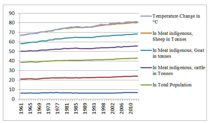
A cursory look at the graph in Figure 2 indicates that temperature change, a proxy for climate change as well as urbanization (urban population growth) were also moving upwards, heading in the same direction with output of the ruminant livestock meat sources. This development buttresses the argument that climate change and variability as well as urbanization can affect the production of livestock. However, this trend analysis is limited in its power to explain whether the association observed here are significant for a valid conclusion.
Long Run Relationship between Urban Population, Total Population, Per Capita Income, Climate Change (Temperature Change) and Livestock Meat Production from Ruminants in Nigeria
The assessment of the long run relationship between demographic (especially urbanization and temperature change) and economic factors (per capita income) on livestock production in this section began with a test for unit root in the series. This was followed by estimation of the long run form (co-integration equations) with the Fully Modified OLS equations (following Phillips PCB, et al. [19] and for each of the livestock product (meat from sheep [lnsheepmt], goat [lngoatmt] and cattle [lncattlemt]) equations. Econometric diagnosis of the estimated residuals was then conducted to see whether there were violations of assumptions of the FMOLS method. When the researcher was satisfied with these outcomes, the estimated parameters were then used for analysis of our hypothesized relationships.
The unit root test results with ADF method are presented in Table 1. The results indicated that all the series were integrated at different levels. One of the series was I (0), five others were I1) and one of them was I(2). In summary the outcome indicates that unit root systems existence in the entire system is not a threat as there are very high chances of co-integration in the entire system.
| Variable | ADF T-Statistics at Levels & P Values | ADF T-Statistic after 1st Differencing and P Value | ADF T-Statistic after 2nd Differencing and P Value | Remark (Order of Integration) |
|---|---|---|---|---|
| lncattlemt | -1.579877 ( p = 0.485) | -9.075728*** (0.000) | NA | I(1) |
| lnsheepmt | -1.581490 (p = 0.4848) | -6.579793 (p = 0.0000) | NA | I(1) |
| lngoatmt | -3.814602*** (p = 0.0050) | NA | NA | I(0) |
| lntotalpop | -0.244494 ( 0.9246) | -6.032507 (p=0.0000) | NA | I(1) |
| lnurbanpop | -1.368525 (p = 0.5904) | -1.994223 (p = 0.2884) | -5.628198*** (p = 0.000) | I(2) |
| lntemp | -1.543888 (p= 0.5034) | -9.332371 (p=0.0000) | NA | I(1) |
| Ln_per_capita_inc | -0.634025 (p = 0.8537 ) | -5.112664 (p = 0.0001) | NA | I (1) |
Table 1: Estimates of Augmented Dickey Fuller test Statistics for all the series used in the Co-integration model.
Given that we have a set of variables whose order of integration are at different levels, one of the most appropriate co-integration regression models to use is the FMOLS model. Eviews provide facilities for conducting this test. The estimates of the FMOLS regression parameters for the three equations are therefore presented in Table 2. The equation test for cointegration with Hansen Parameter Instability test which gave a statistic (Lc) of 0.24 (p>0.2) for the lncattlemt equation; 0.72 (p>0.13) for the lnsheepmt equation and 0.43(p>0.20) for the lngoatmt equation respectively. Since the null hypotheses for these tests held that ‘’ Series are co- integrated’’ we therefore uphold this hypotheses for the three equations and conclude that co-integration exists among the series in each of the models. According to Hansen [26], “the null hypothesis assumes that the parameters are constant.” Hence the existence of steady state relationship between each of the three livestock products and their hypothesized determinants (Including urbanization, per capita income, other variables) is hereby validated. It was found that natural logs of urban population (Coef=1.686, p<0.01), total population (Coef.= -2.588, p<0.05) and per capita income (Coef. = 0.462, p<0.05) significantly determined the long run output levels of meat from cattle production systems in Nigeria. While urban population and per capita income growth exerted positive influences on the output of cattle, total population negatively affected its growth. Since these variables were in natural log forms, the coefficients represent the respective elasticities of supply. These estimated elasticities of income, urban and total population are quite high for beef supply in Nigeria on the long run.
| Dependent Variable | Lnsheepmt | Lnsheepmt | Lngoatmt | ||||||
|---|---|---|---|---|---|---|---|---|---|
| Variable | Coefficient | Std. Error | t-Stat. | Coefficient | Std. Error | t-Stat. | Coefficient | Std. Error | t-Stat. |
| lnper_capita_ income | 0.462 | 0.21 | 2.203** | -0.104 | 0.162 | -0.643 | 0.308 | 0.131 | 2.341** |
| lntotalpop | -2.588 | 1.094 | -2.367** | 1.156 | 0.846 | 1.367 | -5.561 | 0.685 | -8.115*** |
| lnurban_pop | 1.686 | 0.564 | 2.992*** | 0.742 | 0.436 | 1.702* | 4.642 | 0.353 | 13.144*** |
| temperature_ change | 0.214 | 0.145 | 1.474 | 0.053 | 0.112 | 0.474 | 0.111 | 0.091 | 1.213 |
| C | 29.475 | 10.631 | 2.773*** | -21.786 | 8.221 | -2.650** | 36.561 | 6.662 | 5.488*** |
| R-squared | 0.73 | 0.983 | 0.99 | ||||||
| Adjusted R-squared | 0.7 | 0.981 | 0.99 | ||||||
| S.E. of regression | 0.21 | 0.139 | 0.11 | ||||||
| Long-run variance | 0.09 | 0.052 | 0.03 | ||||||
| Lc Statistic | 0.25 | Remark | 0.72 | Remark | 0.43 | Remark | |||
| Prob | > 0.2 | Accept Null (The series are co- integrated) | 0.316 | Accept Null (The series are co- integrated) | >0.2 | Accept Null (The series are co- integrated) |
Table 2: Parameter Estimates of the FMOLS Co-integration Models for the three equations.
For the natural log of sheep equation, only the natural log of urban population (Coef. = 0.742, p>0.10) significantly influenced the variability of its level of production on the long run. The effect was positive and the elasticity of supply with respect to urban population was equally high.
With respect to the variability in natural log of goat products’ (meat) output, natural logs of urban population (Coef. = 4.642, p<0.01), total population (Coef.= -5.561, p<0.01) and per capita income (Coef. = 0.308, p<0.01) were the most significant determinants. The signs of the slope coefficient estimates of the per capita income and urban population for goat production are in line with theoretical expectation. Just as we observed in the case of cattle, only total population growth exhibited a negative relationship with the production of goat meat on the long run in Nigeria. Given that beef and mutton consumption in Nigeria is very high, it is possible that as the total population grew the overall production of these products appeared to be crowded out. This could be further explained by the fact that while prices offered by growing urban areas could trigger increased supply in line with the law of supply [29], rural population growth which is part of total population may not provide such a strong price signal that could increase the of these products, hence this difference. In order to affirm this line of thought further, in the next section, the authors analyzed the relationship between urbanization and prices of the meat products from the three ruminants. However, before we can make valid conclusion with our findings here, there is a need to econometrically ascertain the consistency and reliability of the models’ residual estimates in line with the best econometric principles.
From the findings based on the three estimated equations, we are right to conclude that in empirical terms, the Nigerian case has affirmed the assertion of Sattherwaite, et al. [2] who noted that “urbanization brings major changes in demand for agricultural products both from increases in urban populations and from changes in their diets and demands. It can also bring major challenges for urban and rural food security.’’ These challenges and demand are signals which buoyed the growth of ruminant livestock meat we have observed on the long run in this study.
Further validation of the estimated regression parameters could be viewed from Table 2 and 3. Results of the Jarque-Bera tests in Table 3 indicate that the estimated residuals of the FMOLS models were normally distributed in line with the assumption of OLS. In Table 1, the estimated R-Square (R2) (0.73, 0.98 and 0.99 for sheep, goat and cattle respectively) and the Adjusted R-Squares (0.70, 0.98 and 0.99 for sheep, goat and cattle respectively) of the three equations were very high. These attests to the explanatory power of the model as they imply (for R2s) that the explanatory variables of the models were able to account for 73%, 98% and 99% of the variations in the dependent variables (i.e. natural logs of meats of sheep, goat and cattle equations respectively). Further probe into the forecasting power of the model.
- Statistics Estimated lncattlemt lnsheepmt lngoatmt
- Jarque Bera Test for Residuals Normal Distribution
- JarqueBera Statistics
- 1.35
- Remark
- 2.272
- Remark
- 1.38
- Remark
- Prob.
- 0.509
- Accept Null
- 0.321
- Accept Null
- 0.502
- Accept Null
- Forecasting Power Test Parameters Estimates
- Root Mean Square Error (RMSE)
- 0.206
- 0.131
- 0.107
- Mean Absolute Error(MAPE)
- 1.29
- 0.944
- 0.829
- Theil Inequality Coefficient
- 0.008
- 0.006
- 0.005
- Bias Proportion
- 0
- 0.003
- 0.002
- Covariance Proportion
- 0.977
- 0.993
- 0.993
Table 3: Diagnostic Tests Results on the estimated Co-integration models’ residuals.
Gave results shown for the Root Mean Square Error (RMSE), Mean Absolute Error and the Theil Inequality coefficients in Table 3.These tools are well explained in Gujarati [30]. The very low values of these estimates indicate that their forecasting powers are very high. For instance, the Theil Inequality Coefficients for the three models were almost zero, implying that the difference between the forecasted model and the actual models were almost non-
existent. It is therefore not surprising to see a very high covariance proportion estimates for the models which ranged between 97% to 99% in the three models. The estimates were therefore unbiased and good very fit with excellent forecasting power as they recorded very low bias proportions of almost zero in all the models see the graphs in (Figures 3-5). Tests for serial correlation were also done by estimating the correlogram of the Forecast: LNSHEEPMTF Actual: LNSHEEPMT Forecast sample: 1961 2013 Included observations: 53 Root Mean Squared Error 0.131096 Mean Absolute Error 0.102977 Mean Abs. Percent Error 0.944276 Theil Inequality Coefficient 0.006179 Bias Proportion 0.002765 Variance Proportion 0.004562 Covariance Proportion 0.992673 Figure 3: Estimated and actual lines of residuals with the model forecasting power parameter estimates for lnsheepmt equation.
Forecast: LNGOATMTF Actual: LNGOATMT Forecast sample: 1961 2013 Included observations: 53 Root Mean Squared Error 0.107442 Mean Absolute Error 0.088521 Mean Abs. Percent Error 0.828156 Theil Inequality Coefficient 0.004808 Bias Proportion 0.002326 Variance Proportion 0.002105 Covariance Proportion 0.995570 Figure 4: Estimated and actual lines of residuals with the model forecasting power parameter estimates for lngoatmt equation.
Forecast: LNCATTLEMTF Actual: LNCATTLEMT Forecast sample: 1961 2013 Included observations: 53 Root Mean Squared Error 0.206107 Mean Absolute Error 0.157388 Mean Abs. Percent Error 1.289767 Theil Inequality Coefficient 0.008449 Bias Proportion 0.000011 Variance Proportion 0.023216 Covariance Proportion 0.976773 Figure 5: Estimated and actual lines of residuals with the model forecasting power parameter estimates for lncattlemt equation.
Squared residuals of the three equations. The pattern of the PACF did not indicate presence of serial correlation in the models. According to Gujarati [30] under the null hypothesis of no serial correlation, large Q or Q* implies presence of serial correlation. These was not the case with our Q* estimates.
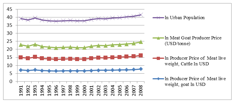
Relationship between Supplier Prices of Meat from Ruminant Livestock Sources and Urban Population Growth
Based on available data at FAOSTAT, the relationship between supplier prices and the producer prices of the three ruminant livestock meat were further assessed as seen in Figure 6. It would be observed that the prices of the three commodities were headed in the same direction with urban population growth. With the high elasticities of supply observed with respect to urban population growth (as inferred from the slope coefficient estimates from the three equations) in Table 2, it is safe to conclude that the urban population, with its higher incomes (purchasing power) relative to the rural counterparts (aggregated into the total population) can drive the prices of livestock (ruminant) meat in the country. However, while the latter drives the supply up by offering higher price incentives to livestock herds (ruminants) suppliers who responded by producing more, it could be that the price signals in the rural population as aggregated in the total population precipitated the negative production levels recorded for the outputs of cattle and goat meat, This probably accounts for the opposing direction of influences of urban population growth and total population growth on the production of cattle and goat meat in the sample.
| Variables | Producer Price Of Meat Live Weight, Cattle In USD | Producer Price Of Meat Live Weight, Sheep In USD | Producer Price Of Meat Live Weight, Goat In USD |
|---|---|---|---|
| Urban Population | R= 0.59 | R= 0.40 | R= 0.57 |
Table 4: Results of Pearson Square Product Moment Correlation for the relationships between urban population and the live weight
The relationship between urban population growth and the producer prices for the three ruminant livestock’s live weights are strong as indicated by the moderate to high correlation coefficients for the three products documented in Table 4.
Conclusion
The study found that urban population growth, total population growth, temperature change growth (climate change proxy), per capita income growth in relationship with historical outputs of meat from cattle, sheep and goat were on the ascent right from 1961 to 2013. However, a major descent was observed in 1986 when the Structural Adjustment Programme was embarked upon in Nigerian economy. This economic programme temporarily reversed the growing tempo of production of ruminant livestock meat in the country before it picked up again after about five years later. A long run relationship was observed between the production of ruminant livestock products (meat from sheep, goat and cattle) and urban population, total population, per capita income and climate change (represented by temperature change). The rest variables exerted significant long run effects on the output of these livestock products. Almost all these determinants, except total population, indicated positive relationship with the production of livestock meat from ruminants. The positive relationship and strong correlations which urban population growth exhibited with the producer prices of these ruminant products enabled us to hypothesize that positive price signals offered by growing urban areas in the country could have triggered the positive relationship between urban population growth and increase in production of the ruminant livestock on the long run.
In view of the fact that urban population growth is driving the production of livestock in the country there are fears that agricultural land for meeting the livestock demand as a result of urban population growth may soon become too scarce. The trend will ultimately pressurize herdsmen and other livestock farmers to adopt more intensive form of livestock production in the future. It will also fuel more crisis beyond the farmers versus herdsmen violent clashes being currently experienced in Nigeria already Nwagboso [31]. Hence Nigerian government and other agricultural stakeholders need to be proactive by preparing the grounds for sustainable livestock intensification as pastoral nomadism being practiced in Nigeria cannot address this challenge. Unfortunately, the newly launched Nigerian Agricultural Promotion Policy 2016-2020, dubbed, The Green Alternative, by the Federal Ministry of Agriculture and Rural Development, FMARD [32] made no policy provision for urban agriculture nor sustainable livestock intensification development. There is therefore, a need toamend this policy to incorporate long term concrete strategies such as allocation of land for ranching and sustainable intensive livestock production in peri-urban areas of the country. Since per capita income in Nigeria is associated with improved livestock production, a policy that will improve the capital base of the livestock farmers such as provision of farm credits to ranch owners in the urban and peri-urban areas should be enforced by Nigerian government and stakeholders who are interested in intervening in this sector. The FMARD (government) should also build capacities of herdsmen and ranch owners to enable them produce high quality meat from their ruminants to meet the growing urban demand and food security need of the country particularly meeting up with the protein requirements of Nigerians. Efforts should be made to broaden the engagement of organized private sector in livestock value chain in Nigeria.
References
-
United Nations (2008) World Urbanization Prospects: The 2007 Revision. United Nations Department of Economic and Social Affairs, Population Division, New York, NY, USA.
-
Satterthwaite D, McGranahan G, Tacoli C(2010) Urbanization and its Implications for Food and Farming. Philosophical Transactions of the Royal Society B: Biological Sciences 365(1554): 2809-2820.
-
Nkrumah B (2018) Edible Backyards: Climate Change and Urban Food (in) Security in Africa. Agriculture & Food Security 7: 45.
-
Fischer G, Winiwarter W, Cao GY, Ermolieva T, Hizsnyik E, et al. (2012) Implications of Population Growth and Urbanization on Agricultural Risks in China. Population and Environment 33: 243-258.
-
Oueslati W, Salanié J, Wu J (2018) Urbanization and Agricultural Productivity: Some Lessons from European Cities. Journal of Economic Geography 19(1): 225-249.
-
Ubesie A, Ibeziakor N (2012) High Burden of Protein- Energy Malnutrition in Nigeria: Beyond the Health Care Setting. Ann Med Health Sci Res 2(1): 66-69.
-
UNDP (United Nations Development Programme) (2015) Sustainable Development Goals.
-
Bourn D, Wint W, Blench R, Woolley E (2018) Nigerian Livestock Resources Survey. Environmental Research Group Oxford, Oxford, United Kingdom.
-
Aydinalp C, Cresser MS (2008) The Effects of Climate Change on Agriculture. J Agric & Environ Sci 3(5): 672- 676.
-
Field CB, Barros VR, Dokken DJ, Mach KJ, Mastrandrea MD (2014) Climate Change 2014-Impacts, Adaptation, and Vulnerability-Part A: Global and Sectoral Aspects. Working Group II Contribution to the Fifth Assessment Report of the Intergovernmental Panel on Climate Change, Cambridge University Press, England.
-
Rojas-Downing MM, Nejadhashemi AP, Woznicki STH (2017) Climate Change and Livestock: Impacts, Adaptation, and Mitigation. Climate Risk Management 16: 145-163.
-
Polley HW, Briske, DD, Morgan JA, Wolter K, Bailey DW, et al. (2013) Climate Change and North American Rangelands: Trends, Projections, and Implications. Rangeland Ecology & Management 66(5): 493-511.
-
Thornton PK , Van de Steeg J, Notenbaert A, Herrrero M (2009) The Impacts of Climate Change on Livestock and Livestock Systems in Developing Countries: A Review of what we know and what we Need to Know. Agricultural Systems.
-
Swain BB, Teufel N (2017) The Impact of Urbanisation on Crop–Livestock Farming System: A Comparative Case Study of India and Bangladesh. Journal of Social and Economic Development 19: 161-180.
-
Sharma VP (2015) Dynamics of Land Use Competition in India: Perceptions and Realities. Indian Institute of Management, India.
-
Thornton P, Herrero M (2010) The Inter-Linkages between Rapid Growth in Livestock Production, Climate Change, and the Impacts on Water Resources, Land Use, and Deforestation. World Bank, USA.
-
Rehman A, Jingdong L, Chandio AA, Hussain I (2017) Livestock Production and Population Census in Pakistan: Determining their Relationship with Agricultural GDP Using Econometric Analysis. Information Processing in Agriculture 4(2): 168-177.
-
World Population Review (2020) Nigeria Population.
-
Phillips PCB, Hansen BE (1990) Statistical Inference in Instrumental Variables Vegression with I(1) Processes. The Review of Economic Studies 57(1): 99-125.
-
Hatanaka M (1996) Time-Series-Based Econometrics, Unit Roots and Co-integration. Oxford University Press, UK.
-
Kao C, Chiang M (2001) On the Estimation and Inference of a Cointegrated Regression in Panel Data. In: Baltagi B, et al. (Eds.), Nonstationary Panels, Panel Cointegration, and Dynamic Panels. Advances in Econometrics, Emerald Group Publishing Limited, England 15: 179-222.
-
Granger CWJ, Newbold (1974) Economic Forecasting: The Atheist’s Viewpoint. In: Renton GA (Ed.), Modeling the Economy. Heinemann, London, pp: 34.
-
Mushtaq R (2011) Augmented Dickey Fuller Test.
-
Dickey D, Fuller W (1979) Distribution of the Estimator for Autoregressive Time Series with a Unit Root. Journal of the American Statistical Association 74: 427-431.
-
Bashier A, Siam AJ (2014) Immigration and Economic Growth in Jordan: FMOLS Approach International. International Journal of Humanities Social Sciences and Education 1(9): 85-92.
-
Hansen BE (1992) Tests for Parameter Instability in Regressions with I(1) Processes. Journal of Business and Economic Statistics 10: 321-335.
-
Phillips PCB (1995) Fully Modied Least Squares and Vector Autoregression. Econometrica 63(5): 1023-1078.
-
Bamidele SI (2000) Structural Adjustment Program and Agricultural Productionin Nigeria (1970 -1996). Degree of Master of Development Economics, Dalhousie University, Canada, pp: 83.
-
Samuelson PA, Nordhaus WD (2005) Economics. Tata McGraw-Hill, New Delhi.
-
Gujarati DN (2004) Basic Econometrics. 4th(Edn.),The McGraw-Hill Companies, NewYork.
-
Nwagboso CI (2018) Nigeria and the challenges of _i_nternal security in the 21st century. European Journal of Interdisciplinary Studies 4(2): 15-33.
-
Federal Ministry of Agriculture and Rural Development (2017) Nigeria’s Agriculture Promotion Policy 2016-2020-Building on the successes of the ATA, closing key gaps. Policy and strategy document. FMARD, Nigeria, pp: 1-59.
- Enhancement of Vegetative Growth and Fruit Yield in Cucumber (Cucumis sativus L.) via Spiritual Blessing (Biofield) Energy Intervention
- Production of Açaí (Euterpe oleracea Mart.) under Different Agroforestry System Management Intensities in Amazonian Floodplain (Varzea) Forests
- Coffee and the Production Region: What is the Secret to the Expression "Quality"?
- Experiential Agripreneurship Training in Sub-Saharan Africa: Integrating a Business Incubator into Postgraduate Livestock Education at the University of Buea
- Advances in Agricultural High-Quality Development
- Linking Compost Residue to ABAGE in Plants - a Short Note