Extrapolation and Interpolation of Information in Computer Science
Proposed method is dealing with multi-dimensional data modeling, extrapolation and interpolation using the set of highdimensional feature vectors. Identification of handwriting, signature, faces or fingerprints need data modeling and each model of the pattern is built by a choice of characteristic key points and multi-dimensional modeling functions. Novel modeling via nodes combination and parameter γ as N-dimensional function enables data parameterization and interpolation for feature vectors. Multi-dimensional data is modelled and interpolated via different functions for each feature: polynomial, sine, cosine, tangent, cotangent, logarithm, exponent, arc sin, arc cos, arc tan, arc cot or power function.
Introduction
The idea of paper is connected with different curve modeling for the same set of curve points (nodes). The problem of multidimensional data modeling appears in many branches of science and industry. Image retrieval, data reconstruction objects identification or pattern recognition is still the open problems in artificial intelligence and computer vision. The paper is dealing with these questions via modeling of high-dimensional data for applications of image segmentation in image retrieval and recognition tasks. Handwriting based author recognition offers a huge number of significant implementations which make it an important research area in pattern recognition. There are so many possibilities and applications of the recognition algorithms that implemented methods have to be concerned on a single problem: retrieval, identification, verification or recognition. This paper is concerned with two parts: image retrieval and recognition tasks. Image retrieval is based on modeling of unknown features via combination of N-dimensional functions for each feature. In the case of biometric writer recognition, each person is represented by the set of modelled letters or symbols. The sketch of proposed method consists of three steps: first handwritten letter or symbol must be modelled by a vector of features (N-dimensional data), then compared with unknown letter and finally there is a decision of identification. Author recognition of handwriting and signature is based on the choice of feature vectors and modeling functions. So high-dimensional data interpolation in handwriting identification [1] is not only a pure mathematical problem but important task in pattern recognition and artificial intelligence such as: biometric recognition, personalized handwriting recognition [2, 3, 4], automatic forensic document examination [5, 6], classification of ancient manuscripts [7]. Also writer recognition [8] in monolingual handwritten texts is an extensive area of study and the methods independent from the language are well-seen [9, 10, 11, 12]. Proposed method represents language-independent and text-independent approach because it identifies the author via a set of letters or symbols from the sample.
Writer recognition methods in the recent years are
going to various directions [13, 14, 15, 16, 17]: writer recognition using multi-script handwritten texts, introduction of new features, combining different types of features, studying the sensitivity of character size on writer identification, investigating writer identification in multi-script environments, impact of ruling lines on writer identification, model perturbed handwriting, methods based on run-length features, the edge-direction and edge-hinge features, a combination of codebook and visual features extracted from chain code and polygonized representation of contours, the autoregressive coefficients, codebook and efficient code extraction methods, texture analysis with Gabor filters and extracting features, using Hidden Markov Model [18] or Gaussian Mixture Model [19]. So hybrid soft computing is essential: no method is dealing with writer identification via N-dimensional data modeling or interpolation and multidimensional points comparing as it is presented in this paper. The paper wants to approach a problem of curve interpolation and shape modeling by characteristic points in handwriting identification [20]. Proposed method relies on nodes combination and functional modeling of curve points situated between the basic set of key points. The functions that are used in calculations represent whole family of elementary functions with inverse functions: polynomials, trigonometric, cyclometric, logarithmic, exponential and power function. Nowadays methods apply mainly polynomial functions, for example Bernstein polynomials in Bezier curves, splines [21] and NURBS. But Bezier curves don’t represent the interpolation method and cannot be used for example in signature and handwriting modeling with characteristic points (nodes). Numerical methods [22, 23, 24] for data interpolation are based on polynomial or trigonometric functions, for example Lagrange, Newton, Aitken and Hermite methods. These methods have some weak sides and are not sufficient for curve interpolation in the situations when the curve cannot be built by polynomials or trigonometric functions [25].
Or
This paper presents novel method of high-dimensional interpolation in hybrid soft computing and takes up method of multidimensional data modeling. The method requires information about data (image, object, curve) as the set of N-dimensional feature vectors. So this paper wants to answer the question: how to retrieve the image using N-dimensional feature vectors and to recognize a handwritten letter or symbol by a set of high-dimensional nodes via hybrid soft computing?
Multidimensional Modeling of Feature Vectors
Proposed method is computing (interpolating) unknown (unclear, noised or destroyed) values of features between two successive nodes (N-dimensional vectors of features) using hybridization of mathematical analysis and numerical methods, Calculated values (unknown or noised features such as coordinates, colors, textures or any coefficients of pixels, voxels and doxels or image parameters) are interpolated and parameterized for real number αi ∈ [0;1] (i = 1,2,…N-1) between two successive values of feature. This method uses the combinations of nodes (N-dimensional feature vectors) p1=(x1,y1,…,z1), p2=(x2,y2,…,z2),…, pn=(xn,yn,…zn) as h(p1,p2,… ,pm) and m=1,2,…n to interpolate unknown value of feature (for example y) for the rest of coordinates:
( ) ( )
1 , 1 , 1,2, 1,
c a x a x c a
z a z k n = × + − × …… = × + − × = … −
, , , , , , 0;1 , 1,2, 1
c c c a F i
N α α γ α = … = … = = … −
∈
1 1 1 1 N N i i i
− − ( ) (1 ) (1 ) ( , ,..., ),
y c y y h p p
p γ γ γ γ = × + − + − ×
1 1 2 k k m
+ [ ] ( ) [ ]
0;1 , , , 0 ( ) ;1
F F a α γ α α = = …
∈ ∈
1 1 i N − (1) Then N-1 features c1,…, cN-1 are parameterized by α1,…, αN-1 between two nodes and the last feature (for example y) is interpolated via formula (1). Of course there can be calculated x(c) or z(c) using (1). Two examples of h (when N = 2) computed for MHR method [26] with good features because of orthogonal rows and columns at Hurwitz-Radon family of matrices:
1 2 1 2 2 1 1 2 ( , ) y y h p p x x x x = + (2)
1 ( , , , ) ( )
h p p p p x x y x x y x x y x x y x x
= + + − + +
1 2 3 4 1 2 1 2 3 3 3 4 1 1 4 3 2 2 1 3
1 ( ) x x y x x y x x y x x y x x
+ + − +
1 2 2 1 4 4 3 4 2 2 3 4 2 2 2 4
The simplest nodes combination is
1 2 ( , ,..., ) 0 m h p p p = (3)
and then there is a formula of interpolation:
1 ) 1( ) ( + − + ⋅ = i i y y c y γ γ .
Formula (1) gives the infinite number of calculations for unknown feature determined by choice of F and h. Nodes combination is the individual feature of each modeled data. Coefficient γ=F(α) and nodes combination h are key factors in data interpolation and object modeling.
N-Dimensional Functions in Modeling
Unknown values of features, settled between the nodes, are computed using (1). Key question is dealing with coefficient γ. The simplest way of calculation means h=0 and γi=αi. Then proposed method represents a linear interpolation. Each interpolation requires specific values of αi and γ in (1) depends on parameters αi and γ in (1) depends on parameters αi ∈ [0;1]:
( ) [ ] [ ] ( ) ( ) 1 , : 0;1 0;1 , 0, ,0 0, 1, ,1 1 N F F F F γ α − = → … = … = And F is strictly monotonic for each αi separately. Coefficient γi are calculated using appropriate function and choice of function is connected with initial requirements and data specifications. Different values of coefficients γi are connected with applied functions Fi(αi). These functions γi = Fi(αi) represent the examples of modeling functions for αi ∈ [0;1] and real number s > 0, i = 1,2,…N-1. Each function is applied for different modelling:
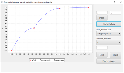
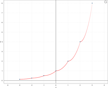
Or any strictly monotonic function between points (0;0) and (1;1). For example interpolations of function y=2x for N = 2, h = 0 and γ = αs with s = 0.8 (Figure 1) is much better than linear interpolation.
( ) ( ) ( ) ( )
,
- / 2 ,
- / 2 , 1
- / 2 , 1
- / 2 ,
s s s s s i i i i i i i i i i
sin sin cos cos = = = = − = −
γ α γ α π γ α π γ α π γ α π ( ) ( ) ( ) ( ) ( )
s s s s s i i i i i i i i i
- / 4 ,
- / 4 , 1 , 1 , 2 –1 ,
α tan tan log log = = = + = + =
γ α π γ α π γ α γ α γ
2 2 ( ) ( ) ( )
= = = − = −( )
s i s s s i i i i i i i
2 /
- , 2 /
- , 1 2 /
- , 1 2 /
· , arcsin arcsin arccos arccos
γ π α γ π α γ π α γ π α ( ) ( ) ( ) ( )
s s s s i i i i i i i i
4 /
- , 4 /
- , / 2 –
- / 4 , / 2
- / 4 ,
arctan arctan ctg ctg = = = = −
γ π α γ π α γ π α π γ π α π ( ) ( )
s s i i i i
2 4 / · , 2 4 / ·
arcctg arcctg = − = −
γ π α γ π α
Functions γi are strictly monotonic for each variable αi ∈ [0;1] as γ = F(α) is N-dimensional modeling function, for example:
i i i i N γ γ γ γ
1
1 1 And every monotonic combination of γi such as ( ) [ ] [ ] ( ) ( ) 1 , : 0;1 0;1 , 0, ,0 0, 1, ,1 1 N F F F F γ α − = → … = … = For example when N = 3 there is a bilinear interpolation:
1 1 2 2 1 2 , , ( ½ ) γ α γ α γ α α = = = + (4)
or a bi-quadratic interpolation:
2 2 2 2 1 1 2 2 1 2 , , ( ½ ) γ α γ α γ α α = = = + (5)
or a bi-cubic interpolation:
3 3 3 3 1 1 2 2 1 2 , , ( ½ ) γ α γ α γ α α = = = + (6)
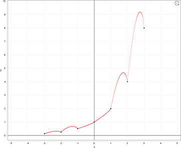
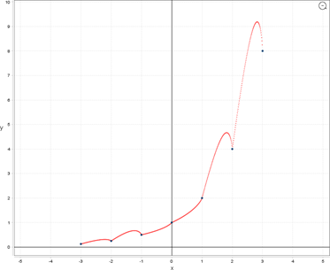
Or others modeling functions γ. Choice of functions γi and value s depends on the specifications of feature vectors and individual requirements. What is very important: two data sets (for example a handwritten letter or signature) may have the same set of nodes (feature vectors: pixel coordinates, pressure, speed, angles) but different h or γ results in different interpolations (Figures 2-4). Here are three examples of reconstruction (Figures 2-4) for N = 2 and four nodes: (-1.5; -1), (1.25; 3.15), (4.4; 6.8) and (8; 7). Formula of the curve is not given. Algorithm of proposed retrieval, interpolation and modeling consists of five steps: first choice of nodes pi (feature vectors), then choice of nodes combination h (p1,p2,…,pm), choice of modeling function γ = F(α), determining values of αi ∈ [0;1] and finally the computations (1).
And other interpolations for the same set of nodes:
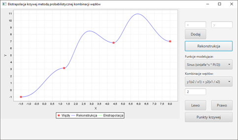
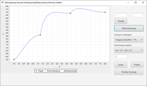
So there are different data reconstructions with different modeling functions. As it can be observed, there is one extremum between two nodes for modeling with h ≠ 0 (Figures 3 & 4). Comparing with polynomial or spline interpolations, there is one very important question: how to avoid extremum between each pair of nodes and how to minimize interpolation error? Generally current methods do not answer this key question. Nowadays methods of interpolations rely mainly on polynomials, especially on cubic splines. It means that there are interpolation polynomials W(x) of degree 3 for every range of two successive interpolation nodes (xi,yi) and (xi+1,yi+1). This method of cubic splines is C2 class – this fact is very important in many applications of cubic interpolation. But second important feature of this method is interpolation error for function f(x):
( ) ( ) 5 ( )( ) , 1
f x W x M x x x x i i
− − − ≤ + sup " , ( )
M x a b f
= ∈ .
x So interpolation error depends on second derivative in the range of nodes [a;b] and this value cannot be estimated in general. Cubic spline can have extremum and may differ from interpolated function f(x) very much. Also interpolation polynomial Wn(x) of degree n (Lagrange or Newton) for n+1 nodes (x0,y0), (x1,y1) … (xn,yn) is connected with unpredictable error in general with calculations of derivative rank n+1:
n M n n ( ) 0 1 1 (n 1)!
+ + ( ) ( )( )...(
) , f x W x x x x
x x x − ≤ − − −
1 . 1 n n + + ∈
sup ( ) M f x
= , x a b Proposed method with h = 0 and α ∈ [0;1] represents formulas as convex combinations of nodes’ coordinates:
1 1 ) (1 ) , ) (1 ( ) y ( k k k k x x y x y α α α α γ γ + + = × + − = × + − And interpolation error in general between two nodes looks as follows:
1 y y k k k ε + − ≤
Proposed method is dealing with such significant features:
- no extremum between two nodes;
- interpolation error does not depend on the value of derivative in the nodes or outside the nodes (even if derivative does not exist);
- interpolated function can be smooth in the nodes (class C1);
- reconstruction of the function that much differs from the shape of polynomial, and not only function but any curve, also closed;
- extrapolation is calculated with the same formulas for α ∈ [0;1];
- the idea of linear interpolation is applied for other modeling functions, not only γ = α1;
- convexity between the nodes is fixed using two modeling functions: γk = αs or γk = sin(αs
- π/2) with real parameter s > 0.
These two kinds of modeling functions are the simplest function, chosen via many calculations as follows:
- γk = αs if convexity is not changing between the nodes (xk,yk) and (xk+1,yk+1);
- γk = sin(αs
- π/2) if convexity is changing between the nodes (xk,yk) and (xk+1,yk+1).
Theorem If
- There are given nodes of continuous function y = f(x): (x0,y0), (x1,y1) … (xn,yn), n ≥ 2;
- There are formulas to calculate values between the nodes:
1 1 ) (1 ) , ) (1 ( ) y ( k k k k x x y x y α α α α γ γ + + = × + − = × + − α ∈ [0;1], k = 2,3…n-1, γk = αs or γk = sin(αs·π/2) with real parameter s > 0; • Three successive nodes are monotonic, for example let’s assume: y0 > y1 > y2 or y0 < y1 < y2 Then there is the method of 2D curve interpolation and extrapolation such as: T.1: There is no extremum between two successive nodes – interpolated function is monotonic in the range of two nodes. T.2: Interpolated curve is class C0 (continuous) or C1 (continuous and smooth). T.3: Interpolation error does not depend on the value of derivative in the nodes or outside the nodes (even if derivative does not exist). T.4: Convexity between two nodes (xk,yk) and (xk+1,yk+1) is fixed using modeling functions γk = αs (if convexity is not changing) or γk = sin(αs·π/2) (if convexity is changing).
T.5: Extrapolation is calculated with the same formulas for α ∈ [0;1].
Proof
T.1: Convex combination to calculate x(α) and y(α) between two nodes with strictly monotonic function γk gives us monotonic interpolation of the curve with no extremum between two nodes. T.2: Interpolated curve is class C0 (continuous) just from definition of x(α) and y(α). Also smooth interpolation between nodes is achieved with the same. Only smooth function in the inner nodes must be proved. Here is shown how to achieve smooth function in the inner nodes – let’s assume then yk ≠ yk+1 for each k. If yk = yk+1 for any k, then according to T.1 there must be the simplest linear interpolation between nodes (xk,yk) and (xk+1,yk+1) and interpolated curve is not smooth in nodes (xk,yk) and (xk+1,yk+1).
For first three monotonic nodes (x0,y0), (x1,y1) and (x2,y2) there are calculations to fix parameter s for modeling function γ1 between nodes (x0,y0) and (x2,y2) interpolating node (x1,y1) inside:
2 0 2 0 (0;1), t (0;1) x x y y x x y y α − − = ∈ = ∈ − − If convexity is not changing between (x0,y0) and (x2,y2), then γ1 = αs and If convexity is changing between (x0,y0) and (x2,y2), then γ1 = sin(αs·π/2) and 2 log ( arcsin ) s t α π =
2 1 2 1 A1 (beginning of the loop in algorithm for k = 2,3…n-1): Having modeling function γ1 between nodes (x0,y0) and (x2,y2), it is possible for any α*→0 calculate
0 2 1 0 1 2 *) * (1 *) , ( ( *) (1 ) y x x y y x α α α α γ γ = × + − = × + − Then left difference quotient c is computed in the node (x2,y2):
( *) ( *) y y c x x
α α − = − Of course if value of derivative in (x2,y2) is known, c = f ’(x2) ≠ 0. Then parameter u is fixed to obtain left (c) and right difference quotient equal in (x2,y2) - it means smooth in this node. If y3 preserves the same monotonicity like y2 and y1 (y1>y2>y3 or y1<y2<y3) then
2
2
3 2 1 (1 *) x x u c y y α − = − − − If y3 does not preserve the same monotonicity like y2 and y1 then (because of different sign of left and right difference quotient) 3 2
3 2
3 2 1 (1 *) x x u c y y α − = + − −
And as it was: if convexity is not changing between (x2,y2) and (x3,y3), then γ2 = αs and log s u α = If convexity is changing between (x2,y2) and (x3,y3), then γ2 = sin(αs·π/2)and
2 log ( arcsin ) s u α π =
So smooth interpolation function in the node (x2,y2) is achieved. And smooth interpolation for next range of nodes (x3,y3) and (x4,y4) is starting like loop A1 for k=3. And so on till last range of nodes (xn-1,yn-1) and (xn,yn) for k = n-1 in A1. T.3: According to T.1 – interpolation error between two nodes for each k is equal:
1 y y k k k ε + ≤ −
T.4: These modeling functions are the simplest functions to achieve convexity changing or not. T.5: Extrapolation left of first node (x0,y0) is done with modeling function γ1 and α>1. Extrapolation right of last node (xn,yn) is done with modeling function γn-1 and α<0. Then modeling function γn-1 must have domain with α<0. If not, there is possibility to define:
1 ( ( ) (1 ) , ) (1 ) y k k k k k k x x x y y α α α α γ γ + = × + − = × + − This theorem describes main features of proposed method.
Image Retrieval via High-dimensional Feature Reconstruction
After the process of image segmentation and during the next steps of retrieval, recognition or identification, there is a huge number of features included in N-dimensional feature vector. These vectors can be treated as “points” in N-dimensional feature space. For example in artificial intelligence there is a high-dimensional search space (the set of states that can be reached in a search problem) or hypothesis space (the set of hypothesis that can be generated by a machine learning algorithm). This paper is dealing with multidimensional feature spaces that are used in computer vision, image processing and machine learning.
Having monochromatic (binary) image which consists of some objects, there is only 2-dimensional feature space (xi,yi) – coordinates of black pixels or coordinates of white pixels. No other parameters are needed. Thus any object can be described by a contour (closed binary curve). Binary images are attractive in processing (fast and easy) but don’t include important information. If the image has grey shades, there is 3-dimensional feature space (xi,yi,zi) with grey shade zi. For example most of medical images are written in grey shades to get quite fast processing. But when there are colour images (three parameters for RGB or other colour systems) with textures or medical data or some parameters, then it is N-dimensional feature space. Dealing with the problem of classification learning for high-dimensional feature spaces in artificial intelligence and machine learning (for example text classification and recognition), there are some methods: decision trees, k-nearest neighbours, perceptron’s, naive Bayes or neural networks methods. All of these methods are struggling with the curse of dimensionality: the problem of having too many features. And there are many approaches to get less number of features and to reduce the dimension of feature space for faster and less expensive calculations. This paper aims at inverse problem to the curse of dimensionality: dimension N of feature space (i.e. number of features) is unchanged, but number of feature vectors (i.e. “points” in N-dimensional feature space) is reduced into the set of nodes. So the main problem is as follows: how to fix the set of feature vectors for the image and how to retrieve the features between the “nodes”? This paper aims in giving the answer of this question.
Grey Scale Image Retrieval Using 3D Method
Binary images are just the case of 2D points (x,y): 0 or 1, black or white, so retrieval of monochromatic images is done for the closed curves (first and last node are the same) as the contours of the objects for N = 2 and examples as (Figures 1-4). Grey scale images are the case of 3D points (x,y,s) with s as the shade of grey. So the grey scale between the nodes p1=(x1,y1,s1) and p2=(x2,y2,s2) is computed with γ = F(α) = F(α1,α2) as (1) and for example (4-6) or others modeling functions γi. As the simple example two successive nodes of the image are: left upper corner with coordinates p1=(x1,y1,2) and right down corner p2=(x2,y2,10). The image retrieval with the grey scale 2-10 between p1 and p2 looks as follows for a bilinear interpolation (4) (Figure 5):
| 2 | 3 | 4 | 5 | 6 | 7 | 8 | 9 | 10 |
|---|---|---|---|---|---|---|---|---|
| 2 | 3 | 4 | 5 | 6 | 7 | 8 | 9 | 10 |
| 2 | 3 | 4 | 5 | 6 | 7 | 8 | 9 | 10 |
| 2 | 3 | 4 | 5 | 6 | 7 | 8 | 9 | 10 |
| 2 | 3 | 4 | 5 | 6 | 7 | 8 | 9 | 10 |
| 2 | 3 | 4 | 5 | 6 | 7 | 8 | 9 | 10 |
| 2 | 3 | 4 | 5 | 6 | 7 | 8 | 9 | 10 |
| 2 | 3 | 4 | 5 | 6 | 7 | 8 | 9 | 10 |
| 2 | 3 | 4 | 5 | 6 | 7 | 8 | 9 | 10 |
| 2 | 2 | 2 | 2 | 2 | 2 | 2 | 2 | 2 |
| 2 | 3 | 3 | 3 | 3 | 3 | 3 | 3 | 3 |
| 2 | 3 | 4 | 4 | 4 | 4 | 4 | 4 | 4 |
| 2 | 3 | 4 | 5 | 5 | 5 | 5 | 5 | 5 |
| 2 | 3 | 4 | 5 | 6 | 6 | 6 | 6 | 6 |
| 2 | 3 | 4 | 5 | 6 | 7 | 7 | 7 | 7 |
| 2 | 3 | 4 | 5 | 6 | 7 | 8 | 8 | 8 |
| 2 | 3 | 4 | 5 | 6 | 7 | 8 | 9 | 9 |
| 2 | 3 | 4 | 5 | 6 | 7 | 8 | 9 | 10 |
The feature vector of dimension N = 3 is called a voxel.
Colour Image Retrieval
Colour images in for example RGB colour system (r,g,b) are the set of points (x,y,r,g,b) in a feature space of dimension N = 5. There can be more features, for example texture t, and then one pixel (x,y,r,g,b,t) exists in a feature space of dimension N = 6. But there are the sub-spaces of a feature space of dimension N1 < N, for example (x,y,r), (x,y,g), (x,y,b) or (x,y,t) are points in a feature sub-space of dimension N1=3. Reconstruction and interpolation of color coordinates or texture parameters is done like in section 3.1 for dimension N = 3. Appropriate combination of α1 and α2 le0ads to modeling of colour r,g,b or texture t or another feature between the nodes. And for example (x,y,r,t), (x,y,g,t), (x,y,b,t)) are points in a feature sub-space of dimension N1=4 called doxels. Appropriate combination of α1, α2 and α3 leads to modeling of texture t or another feature between the nodes. For example colour image, given as the set of doxels (x,y,r,t), is described for coordinates (x,y) via pairs (r,t) interpolated between nodes (x1,y1,2,1) and (x2,y2,10,9) (Figure 6) as follows:
| 2,1 | 3,1 | 4,1 | 5,1 | 6,1 | 7,1 | 8,1 | 9,1 | 10,1 |
|---|---|---|---|---|---|---|---|---|
| 2,2 | 3,2 | 4,2 | 5,2 | 6,2 | 7,2 | 8,2 | 9,2 | 10,2 |
| 2,3 | 3,3 | 4,3 | 5,3 | 6,3 | 7,3 | 8,3 | 9,3 | 10,3 |
| 2,4 | 3,4 | 4,4 | 5,4 | 6,4 | 7,4 | 8,4 | 9,4 | 10,4 |
| 2,5 | 3,5 | 4,5 | 5,5 | 6,5 | 7,5 | 8,5 | 9,5 | 10,5 |
| 2,6 | 3,6 | 4,6 | 5,6 | 6,6 | 7,6 | 8,6 | 9,6 | 10,6 |
| 2,7 | 3,7 | 4,7 | 5,7 | 6,7 | 7,7 | 8,7 | 9,7 | 10,7 |
| 2,8 | 3,8 | 4,8 | 5,8 | 6,8 | 7,8 | 8,8 | 9,8 | 10,8 |
| 2,9 | 3,9 | 4,9 | 5,9 | 6,9 | 7,9 | 8,9 | 9,9 | 10,9 |
So dealing with feature space of dimension N and using novel method there is no problem called “the curse of dimensionality” and no problem called “feature selection” because each feature is important. There is no need to reduce the dimension N and no need to establish which feature is “more important” or “less important”. Every feature that depends from N1-1 other features can be interpolated (reconstructed) in the feature sub-space of dimension N1 < N via proposed method. But having a feature space of dimension N and using author’s method there is another problem: how to reduce the number of feature vectors and how to interpolate (retrieve) the features between the known vectors (called nodes). Difference between two given approaches (the curse of dimensionality with feature selection and author’s interpolation) can be illustrated as follows. There is a feature matrix of dimension N x M: N means the number of features (dimension of feature space) and M is the number of feature vectors (interpolation nodes) – columns are feature vectors of dimension N. One approach (Figure 7): the curse of dimensionality with feature selection wants to eliminate some rows from the feature matrix and to
reduce dimension N to N1 < N. Second approach (Figure 8) for this method wants to eliminate some columns from the feature matrix and to reduce dimension M to M1 < M.
| 2 | 2 | 2 | 2 | 2 | 2 | 2 | 2 | 2 |
| 2 | 3 | 3 | 3 | 3 | 3 | 3 | 3 | 3 |
| 2 | 3 | 4 | 4 | 4 | 4 | 4 | 4 | 4 |
| 2 | 3 | 4 | 5 | 5 | 5 | 5 | 5 | 5 |
| 2 | 3 | 4 | 5 | 6 | 6 | 6 | 6 | 6 |
| 2 | 3 | 4 | 5 | 6 | 7 | 7 | 7 | 7 |
| 2 | 2 | 2 | 2 | 2 | 2 | 2 | 2 | 2 |
|---|---|---|---|---|---|---|---|---|
| 2 | 3 | 3 | 3 | 3 | 3 | 3 | 3 | 3 |
| 2 | 3 | 4 | 4 | 4 | 4 | 4 | 4 | 4 |
| 2 | 3 | 4 | 5 | 5 | 5 | 5 | 5 | 5 |
| 2 | 3 | 4 | 5 | 6 | 6 | 6 | 6 | 6 |
| 2 | 3 | 4 | 5 | 6 | 7 | 7 | 7 | 7 |
| 2 | 3 | 4 | 5 | 6 | 7 | 8 | 8 | 8 |
| 2 | 3 | 4 | 5 | 6 | 7 | 8 | 9 | 9 |
| 2 | 3 | 4 | 5 | 6 | 7 | 8 | 9 | 10 |
| 2 | 2 | 2 | 2 | 2 | 2 | 2 |
|---|---|---|---|---|---|---|
| 2 | 3 | 3 | 3 | 3 | 3 | 3 |
| 2 | 3 | 4 | 4 | 4 | 4 | 4 |
| 2 | 3 | 4 | 5 | 5 | 5 | 5 |
| 2 | 3 | 4 | 5 | 6 | 6 | 6 |
| 2 | 3 | 4 | 5 | 6 | 7 | 7 |
| 2 | 3 | 4 | 5 | 6 | 7 | 8 |
| 2 | 3 | 4 | 5 | 6 | 7 | 8 |
| 2 | 3 | 4 | 5 | 6 | 7 | 8 |
So after feature selection (Figure 7) there are nine feature vectors (columns): M = 9 in a feature sub-space of dimension N1 = 6 < N (three features are fixed as less important and reduced). But feature elimination is a very unclear matter. And what to do if every feature is denoted as meaningful and then no feature are to be reduced? For this method (Figure 8) there are seven feature vectors (columns): M1 = 7 < M in a feature space of dimension N = 9. Then no feature is eliminated and the main problem is dealing with interpolation or extrapolation of feature values, like for example image retrieval (Figures 5 & 6).
Recognition Tasks via High-Dimensional Feature Vectors’ Interpolation
The process of biometric recognition and identification consists of three parts: pre-processing, image segmentation with feature extraction and recognition or verification. Pre-processing is a common stage for all methods with binarization, thinning, size standardization. Proposed online approach is based on 2D curve modeling and multi-dimensional feature vectors’ interpolation. Feature extraction gives the key points (nodes as N-dimensional feature vectors) that are used in curve reconstruction and identification. Proposed method enables signature and handwriting recognition, which is used for biometric purposes, because human signature or handwriting consists of non-typical curves and irregular shapes (for example Figures 2-4). The language does not matter because each symbol is treated as a curve. This process of recognition consists of three parts:
1. Before Recognition: continual and never-ending building the data basis: patterns’ modeling – choice of nodes combination, function (1) and values of features (pen pressure, speed, pen angle etc.) appearing in high dimensional feature vectors for known signature or handwritten letters of some persons in the basis; 2. Feature Extraction: unknown author – fixing the values in feature vectors for unknown signature or handwritten words: N-dimensional feature vectors (x,y,p,s,a,t) with x,y-points’ coordinates, p-pen pressure, s-speed of writing, a- pen angle or any other features t; 3. The Results: Recognition or identification - comparing the results of interpolation for known patterns from the data basis with features of unknown object.
Signature Modeling and Multidimensional Recognition
Human signature or handwriting consists mainly of non- typical curves and irregular shapes. So how to model two- dimensional handwritten characters via author’s method? Each model has to be described (1) by the set of nodes, nodes combination h and a function γ=F(α) for each letter. Other features in multi-dimensional feature space are not visible but used in recognition process (for example p-pen pressure, s-speed of writing, a-pen angle). Less complicated models can take h(p1,p2,…,pm) = 0 and then the formula of interpolation (1) looks as follows:
1 ( ) (1 ) i i y c y y γ γ + = × + − (7)
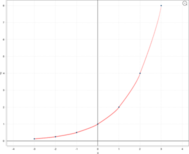
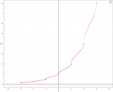
Formula (7) represents the simplest linear interpolation if γ = α. Here are some examples of non-typical curves and irregular shapes as the whole signature or a part of signature, reconstructed via proposed method for y=2x and seven nodes (x,y) like (Figure 1):
| LP | X | Y |
|---|---|---|
| 1 | -3.0 | 0.125 |
| 2 | -2.0 | 0.25 |
| 3 | -1.0 | 0.5 |
| 4 | 0.0 | 1.0 |
| 5 | 1.0 | 2.0 |
| 6 | 2.0 | 4.0 |
| 7 | 3.0 | 8.0 |
And two other interpolations for the same set of nodes:

So there are different data reconstructions with different modeling functions. Other interpolations for the same set of nodes and combination h=0 are as follows:
.
(Figures 9-13) are two-dimensional subspace of N-dimensional feature space, for example (x,y,p,s,a,t) when N = 6. If the recognition process is working “offline” and features p-pen pressure, s-speed of writing, a- pen angle or another feature t are not given, the only information before recognition is situated in x,y points’ coordinates.
After pre-processing (binarization, thinning, size standardization), feature extraction is second part of biometric identification. Choice of characteristic points (nodes) for unknown letter or handwritten symbol is a crucial factor in object recognition. The range of coefficients x has to be the same like the x range in the basis of patterns. When the nodes are fixed, each coordinate of every chosen point on the curve (x0 c,y0 c), (x1 c,y1 c),…, (xM c,yM c) is accessible to be used for comparing with the models. Then modeling function γ = F(α) and nodes combination h have to be taken from the basis of modelled letters to calculate appropriate second coordinates yi (j) of the pattern Sj for first coordinates xi c, i=0,1,…,M. After interpolation it is possible to compare given handwritten symbol with a letter in the basis of patterns. Comparing the results of this interpolation for required second coordinates of a model in the basis of patterns with points on the curve (x0 c,y0 c), (x1 c,y1 c),…, (xM c,yM c), one can say if the letter or symbol is written by person P1, P2 or another. The comparison and decision of recognition is done via minimal distance criterion. Curve points of unknown handwritten symbol are: (x0 c,y0 c), (x1 c,y1 c),…, (xM c,yM c). The criterion of recognition for models Sj = {(x0 c,y0 (j)), (x1 c,y1 (j)),…, (xM c,yM (j)), j=0,1,2,3…K} is given as:
M M
2 ) ( → − ∑ =
) ( → − ∑ =
j i c i y y
j i c i y y (8)
min or min
0 i
0 i Minimal distance criterion helps us to fix a candidate for unknown writer as a person from the model Sj in the basis.
If the recognition process is “online” and features p-pen pressure, s-speed of writing, a- pen angle or some feature t are given, then there is more information in the process of author recognition, identification or verification in a feature space (x,y,p,s,a,t) of dimension N = 6 or others. Some person may know how the signature of another man looks like (for example Figures 2-4 or Figures 9-13), but other extremely important features p,s,a,t are not visible. Dimension N of a feature space may be very high, but this is no problem. As it is illustrated (Figures 7 & 8) the problem connected with the curse of dimensionality with feature selection does not matter. There is no need to fix which feature is less important and can be eliminated. Every feature is very important and each of them can be interpolated between the nodes using author’s high-dimensional interpolation. For example pressure of the pen p differs during the signature writing and p is changing for particular letters or fragments of the signature. Then feature vector (x,y,p) of dimension N1 = 3 is dealing with p interpolation at the point (x,y) via modeling functions (4)-(6) or others. If angle of the pen a differs during the signature writing and a is changing for particular letters or fragments of the signature, then feature vector (x,y,a) of dimension N1 = 3 is dealing with a interpolation at the point (x,y) via modeling functions (4)-(6) or others. If speed of the writing s differs during the signature writing and s is changing for particular letters or fragments of the signature, then feature vector (x,y,s) of dimension N1 = 3 is dealing with s interpolation at the point (x,y) via modeling functions (4)-(6) or others. This 3D interpolation is the same like in section 3.1 grey scale image retrieval but for selected pairs (α1, α2) – only for the points of signature between (x1,y1,2) and (x2,y2,10):
| 2 | 3 | 0 | 0 | 0 | 0 | 0 | 0 | 0 |
|---|---|---|---|---|---|---|---|---|
| 0 | 0 | 4 | 5 | 0 | 0 | 0 | 0 | 0 |
| 0 | 0 | 0 | 0 | 6 | 0 | 0 | 0 | 0 |
| 0 | 0 | 0 | 0 | 0 | 7 | 0 | 0 | 0 |
| 0 | 0 | 0 | 0 | 0 | 0 | 8 | 0 | 0 |
| 0 | 0 | 0 | 0 | 0 | 0 | 0 | 9 | 0 |
| 0 | 0 | 0 | 0 | 0 | 0 | 0 | 0 | 10 |
| 0 | 0 | 0 | 0 | 0 | 0 | 0 | 0 | 10 |
| 0 | 0 | 0 | 0 | 0 | 0 | 0 | 0 | 10 |
If a feature sub-space is dimension N1 = 4 and feature vector is for example (x,y,p,s), then 4D interpolation is the same like in section 3.2 colour image retrieval but for selected pairs (α1, α2) – only for the points of signature between (x1,y1,2,1) and (x2,y2,10,9):
| 2,1 | 3,1 | 0 | 0 | 0 | 0 | 0 | 0 | 0 |
|---|---|---|---|---|---|---|---|---|
| 0 | 0 | 4,2 | 5,2 | 0 | 0 | 0 | 0 | 0 |
| 0 | 0 | 0 | 0 | 6,3 | 0 | 0 | 0 | 0 |
| 0 | 0 | 0 | 0 | 0 | 7,4 | 0 | 0 | 0 |
| 0 | 0 | 0 | 0 | 0 | 0 | 8,5 | 0 | 0 |
| 0 | 0 | 0 | 0 | 0 | 0 | 0 | 9,6 | 0 |
| 0 | 0 | 0 | 0 | 0 | 0 | 0 | 0 | 10,7 |
| 0 | 0 | 0 | 0 | 0 | 0 | 0 | 0 | 10,8 |
| 0 | 0 | 0 | 0 | 0 | 0 | 0 | 0 | 10,9 |
If a feature sub-space is dimension N1 = 5 and feature vector is for example (x,y,p,s,a), then 5D interpolation is the same like in section 3.2 colour image retrieval but for selected pairs (α1, α2) – only for the points of signature between (x1,y1,2,1,30) and (x2,y2,10,9,60):
| 2,1,30 | 3,1,30 | 0 | 0 | 0 | 0 | 0 | 0 | 0 |
|---|---|---|---|---|---|---|---|---|
| 0 | 0 | 4,2,32 | 5,2,34 | 0 | 0 | 0 | 0 | 0 |
| 0 | 0 | 0 | 0 | 6,3,37 | 0 | 0 | 0 | 0 |
| 0 | 0 | 0 | 0 | 0 | 7,4,43 | 0 | 0 | 0 |
| 0 | 0 | 0 | 0 | 0 | 0 | 8,5,45 | 0 | 0 |
| 0 | 0 | 0 | 0 | 0 | 0 | 0 | 9,6,46 | 0 |
| 0 | 0 | 0 | 0 | 0 | 0 | 0 | 0 | 10,7,53 |
| 0 | 0 | 0 | 0 | 0 | 0 | 0 | 0 | 10,8,56 |
| 0 | 0 | 0 | 0 | 0 | 0 | 0 | 0 | 10,9,60 |
(Figures 14-16) are the examples of denotation for the features that are not visible during the signing or handwriting but very important in the process of “online” recognition, identification or verification. Even if from technical reason or other reasons only some points of signature or handwriting (feature nodes) are given in the process of “online” recognition, identification or verification, the values of features between nodes are computed via multidimensional author’s interpolation like for example between (x1,y1,2) and (x2,y2,10) on (Figure 14), between (x1,y1,2,1) and (x2,y2,10,9) on (Figure 15) or between (x1,y1,2,1,30) and (x2,y2,10,9,60) on (Figure 16). Reconstructed features are compared with the features in the basis of patterns like parameter y in (8) and appropriate criterion gives the result.
So persons with the parameters of their signatures are allocated in the basis of patterns. The curve does not have to be smooth at the nodes because handwritten symbols are not smooth. The range of coefficients x has to be the same for all models because of comparing appropriate coordinates y. Every letter or a part of signature is modelled via three factors: the set of high-dimensional feature nodes, modeling function γ=F(α) and nodes combination h. These three factors are chosen individually for each letter or a part of signature therefore this information about modelled curves seems to be enough for specific multidimensional curve interpolation and handwriting identification. What is very important, novel N-dimensional modeling is independent of the language or a kind of symbol (letters, numbers, characters or others). One person may have several patterns for one handwritten letter or signature. Summarize: every person has the basis of patterns for each handwritten letter or symbol, described by the set of feature nodes, modeling function γ = F(α) and nodes combination h. Whole basis of patterns consists of models Sj for j = 0,1,2,3…K. Proposed interpolation is used for parameterization and reconstruction of curves in the plane.
Conclusion
The author’s method enables interpolation and modeling of high-dimensional data using features’ combinations and different coefficients γ: polynomial, sinusoidal, cosinusoidal, tangent, cotangent, logarithmic, exponential, arc sin, arc cos, arc tan, arc cot or power function. Functions for γ calculations are chosen individually at each data modeling and it is treated as N-dimensional function: γ depends on initial requirements and features’ specifications. Novel method leads to data interpolation as handwriting or signature identification and image retrieval via discrete set of feature vectors in N-dimensional feature space. So this method makes possible the combination of two important problems: interpolation and modeling in a matter of image retrieval or writer identification. Main features of the method are: this interpolation develops a linear interpolation in multidimensional feature spaces into other functions as N-dimensional functions; nodes combination and coefficients γ are crucial in the process of data parameterization and interpolation: they are computed individually for a single feature; modeling of closed curves.
References
-
Marti UV, Bunke H (2002) The IAM-database: an English sentence database for offline handwriting recognition. Int J Doc Anal Recognit 5(1): 39-46.
-
Djeddi C, Meslati LS (2010) A texture based approach for Arabic writer identification and verification. In: International Conference on Machine and Web Intelligence pp: 115-120.
-
Djeddi C, Meslati LS (2011) Artificial immune recognition system for Arabic writer identification. International Symposium on Innovation in Information and Communication Technology pp: 159-165.
-
Nosary A, Heutte L, Paquet T (2004) Unsupervised writer adaption applied to handwritten text recognition. Pattern Recogn Lett 37(2): 385-388.
-
Van EM, Vuurpijl LG, Franke K, Schomaker LRB (2005) The WANDA measurement tool for forensic document examination. J Forensic Doc Exam 16: 103-118.
-
Schomaker L, Franke K, Bulacu M (2007) Using codebooks of fragmented connected-component contours in forensic and historic writer identification. Pattern Recogn Lett 28(6): 719-727.
-
Siddiqi I, Cloppet F, Vincent N (2009) Contour based features for the classification of ancient manuscripts. Conference of the International Graphonomics Society pp: 226-229.
-
Garain U, Paquet T (2009) Off-line multi-script writer identification using AR coefficients. International Conference on Document Analysis and Recognition pp: 991-995.
-
Bulacu M, Schomaker L, Brink A (2007) Text-independent writer identification and verification on off-line Arabic handwriting. International Conference on Document Analysis and Recognition pp: 769-773.
-
Ozaki M, Adachi Y, Ishi N (2006) Examination of effects of character size on accuracy of writer recognition by new local arc method. International Conference on Knowledge-Based Intelligent Information and Engineering Systems pp: 1170-1175.
-
Chen J, Lopresti D, Kavallieratou E (2010) the impact of ruling lines on writer identification. International Conference on Frontiers in Handwriting Recognition pp: 439-444.
-
Chen J, Cheng W, Lopresti D (2011) Using perturbed handwriting to support writer identification in the presence of severe data constraints. Document Recognition and Retrieval pp: 1-10.
-
Galloway MM (1975) Texture analysis using gray level runs lengths. Comput Graphics Image Process. 4(2): 172-179.
-
Siddiqi I, Vincent N (2010) Text independent writer recognition using redundant writing patterns with contour-based orientation and curvature features. Pattern Recogn Lett 43(11): 3853-3865.
-
Ghiasi G, Safabakhsh R (2013) Offline text-independent writer identification using codebook and efficient code extraction methods. Image and Vision Computing 31(5): 379-391.
-
Shahabinejad F, Rahmati M (2007) a new method for writer identification and verification based on Farsi/ Arabic handwritten texts. Ninth International Conference on Document Analysis and Recognition pp: 829-833.
-
Schlapbach A, Bunke H (2007) A writer identification and verification system using HMM based recognizers. Pattern Anal Appl 10(1): 33-43.
-
Schlapbach A, Bunke H (2004) Using HMM based recognizers for writer identification and verification. 9th Int Workshop on Frontiers in Handwriting Recognition pp: 167-172.
-
Schlapbach A, Bunke H (2006) Off-line writer identification using Gaussian mixture models. International Conference on Pattern Recognition pp: 992-995.
-
Bulacu M, Schomaker L (2007) Text-independent writer identification and verification using textural and allographic features. IEEE Trans Pattern Anal Mach Intell 29(4): 701-717.
-
Schumaker LL (2007) Spline Functions: Basic Theory. Cambridge Mathematical Library.
-
Collins GW (2003) Fundamental Numerical Methods and Data Analysis. Case Western Reserve University.
-
Chapra SC (2012) Applied Numerical Methods. McGraw- Hill.
-
Ralston A, Rabinowitz P (2001) a First Course in Numerical Analysis. Dover Publications.
-
Zhang D, Lu G (2004) Review of Shape Representation and Description Techniques. Pattern Recognition 1(37): 1-19.
-
Jakobczak DJ (2014) 2D Curve Modeling via the Method of Probabilistic Nodes Combination - Shape Representation, Object Modeling and Curve Interpolation-Extrapolation with the Applications. Lambert Academic Publishing.
- Revolutionizing Property Measurement Through Artificial Intelligence: The Journey of PropertyMeasure.ai
- AI Infused Business Model Innovation for Competitive Advantage in the Era of Big Data and Digital Transformation
- Use of CPM/PERT in the Effort to Eradicate Polio
- Integrated Multimodal Deep Learning Framework for Early Detection of Mouth Cancer Using CT Imaging and Clinical Symptom Analysis
- Artificial Intelligence in Medical Robotics and Assistance: An Overview
- Server Migration with Multipath-QUIC