Comparative Analysis of the Spread of the COVID 19 Epidemic in Berlin and New York City Based on a Computational Model
A simple calculation method is proposed based on the approximate spread model of COVID 19. A comparison of the calculation results for NYC and Berlin with observational data on the development of the epidemic in these cities shows a good match. The calculation method uses two empirical coefficients. One of them for a certain strain of the virus depends only on the population size. The second coefficient is determined by the intensity of contacts between carriers of the virus. The correlation of this coefficient with quarantine conditions and socio-demographic characteristics of cities makes it possible to use the proposed methodology not only for calculating epidemic growth but also for operational forecasting. The analysis of the passage of different epidemic waves in NYC and Berlin allows us to draw some preliminary conclusions about the effectiveness of epidemic control in both cities. The proposed model can be an additional simple and reliable tool for city administrations to continuously monitor the development of the epidemic, especially in its early stages.
Introduction
A large number of studies have been devoted to studies related to the intensity of the spread of the СOVID -19 epidemic. Roughly speaking, in terms of their methodological approach, either deterministic or stochastic models are the basis for describing epidemic growth. However, both classes of models can only be implemented by numerical methods and, most importantly, by using a large number of empirical coefficients. This circumstance makes it difficult to use such models for practical use as a means of constantly controlling the epidemic and analyzing possible results in the choice of various strategies for combating the spread of infection, but also to become an operative tool for predicting the possible consequences of management decisions. This paper is devoted to an attempt to create a rather simple and at the same time reliable model.
Methodology
The basis of the developed model of epidemic spreading is the system of equations widely used, for example, in SIR models [1]. The joint solution of these equations can only be obtained by numerical methods. In the future, the general trend in the development of models will be mainly reduced to their complication and introduction of more and more coefficients (e.g., [2]). At the same time, in conditions where the majority of the population has not developed immunity against a certain type of virus and the number of infected patients is significantly lower than the potential number of people with a real possibility of infection, a simplified analytical model can be used. The basic equations of the model can be written as [3]:
100 exp[ (1 e )] t r o s k i i N
λ λ $$ i = i _ {o} + \frac {1 0 0}{N} * \exp \left[ \frac {k _ {r}}{\lambda} \left(1 - \mathrm {e} ^ {- \lambda}\right) \right. $$ (1) In which: i - Number of infected persons per one inhabitant of the settlement as a percentage, 𝑁𝑠 - Population of the country, city or region for which the calculation is performed, 𝑘𝑟 - Coefficient of virus transmission rate, which depends on both the type of strain and size of the area for which the calculation is performed. λ - Intensity factor of decrease in contacts of infected patients with persons who potentially can get infected by means of quarantine and other preventive measures.
For the strain type of the first wave of the epidemic under consideration, similarly to that of the second wave, we assume that this coefficient can be estimated by a simple formula [3]:
$$ K _ {r} = 0. 4 - 0. 0 3 5 \ln \left(\frac {3 . 6}{N r} * 1 0 ^ {6}\right) $$
(2) The coefficients in (1) were obtained by recalculating the calculated conditions of the city of Berlin to the conditions of other populated areas. Thus, the maximum number of infected people for a given locality decreases with the increase in the quarantine severity, characterized by the coefficient λ. The value of the maximum daily increase in the number of infected can be found by equating the second derivative of equation (1) [4] to zero.
max 100 exp( 1) $$ \Delta i _ {\max } = \frac {1 0 0}{N _ {s}} \lambda \exp \left(\frac {k}{\lambda} - 1\right) \tag {3} $$ s Accordingly, the time of the maximum daily increase in the number of infected people, counting from the beginning of quarantine:
λ ln( ) max k t $$ = - \frac {\ln \left(\frac {k}{\lambda}\right)}{\lambda} (4) $$
Results
Comparison of Berlin and New York
These dependencies were initially used to calculate the initial stage of the first wave of the coronavirus epidemic in a number of cities and countries [5]. Now that the first wave has already been fully completed, we can perform a more complete analysis of its features. Let us consider, for example, the passage of the first wave in Berlin (Germany) and New York. The choice of these two cities for comparison is related to the fact that, as it is commonly believed, Berlin turned out to be one of the most successful large cities, which managed to prevent active growth of the first epidemic wave, while in New York the first epidemic wave reached very high values.
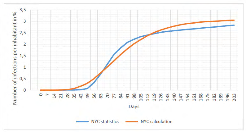
Figure 1 shows a comparison of statistical data [6] with the results of calculations for the first wave of the epidemic in New York City. The calculations were performed for the value of coefficient λ = 0.0345 1/day. The second coefficient in the calculated dependence (1) was determined by formula (2) and was equal to Kr = 0.43 1/day for New York. Despite a good formal coincidence of the calculated and observed data (correlation coefficient above 0.95), we should note a number of their fundamental differences. The calculated curve runs much more gently in the initial stage of the epidemic, however, in the second stage of this wave, the introduction of sufficiently strict quarantine methods managed to sharply reduce the rate of further spread of the epidemic of particular interest is the study of the initial stage of the epidemic. First of all, it should be noted that quarantine was introduced in the city with a significant delay, only 63 days from the beginning of the epidemic. At that point in time, the number of detected infections, even in conditions of low coverage by testing, was already reaching about 1% of the city population. The weekly increase in infected city residents at this point in time reached more than 37000 people, which is over 5000 people a day or ∆imax = 0,065%. Positive results from the introduction of quarantine could only really be observed on the 77th day, when the rate of the spread of the epidemic began to decrease.
Let us estimate both the time of the maximum rate of epidemic growth and the value of this rate itself. By equating ∆imax = 0,065%. Into (3), we obtain, after solving this transcendental equation, the coefficient λ = 0.033 1/day. Correspondingly, at this value of λ, we find in combination with (4) that such a high growth rate of the epidemic should arrive approximately in 78 days after its start, which is fully confirmed by observations. The most important thing however, is to estimate the expected further development of this epidemic wave if emergency measures for its localization had not been introduced. The calculations according to the equation (1) with the obtained coefficient λ = 0.033 1/ day show that in such a situation the maximum number of infections in the city would have reached about 500000 people or about 6% of the city population. Of course, it would be extremely difficult for any city health care system to cope with such a high increase in the number of cases in a relatively short period of time. The main conclusion that follows from the above analysis is the need to strictly control the possible emergence of an epidemic and to take the most urgent measures to eliminate it at the initial stage.
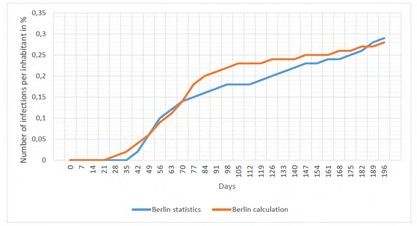
As an example of such successful tactics to combat the epidemic in its early stages, consider the passage of the first wave in Berlin, Germany. The first restrictive measures contributing to reducing the growth of the epidemic in Berlin were taken by the city administration already about a month after the beginning of the epidemic [7]. It is difficult to judge the exact number of infected persons at this point in time due to the small number of tests performed. However, the relative number of those infected at this point in time, as can be seen in Figure 2, did not exceed 0.05% [6]. The maximum daily increase in infections in Berlin during the first wave was about 200 people per day or ∆imax= 0.0055 %. Using ratio (3), that this rate of epidemic growth corresponds to the coefficient λ= 0.042 1/day, we find the maximum number of infected people in the case that no more stringent further measures were taken to limit epidemic growth, including limiting the operation of enterprises in the city. Estimates shows that in such a case we could expect that the number of infected would reach 15000, while in reality it did not exceed 7000 people.
Second and Third Wave’s Analysis
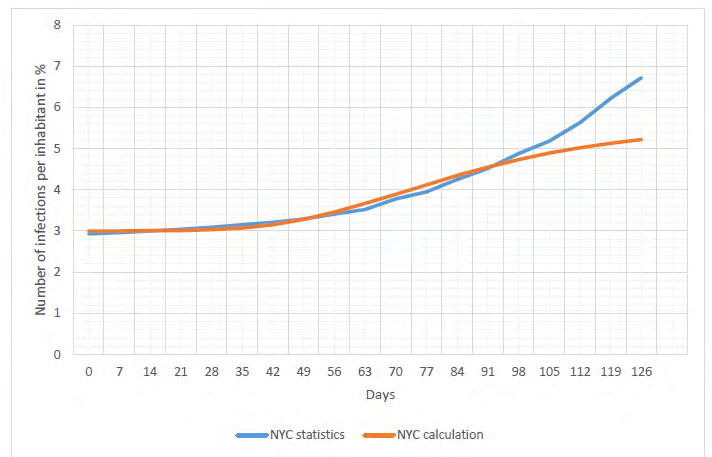
A new sharp increase in infections was registered in most countries in mid- and late- September 2020, when a new wave of the virus began to spread actively. If we assume that this sharp increase in the epidemic was caused by a new strain of the virus, and then we can consider this autumn- winter wave as a new epidemic. The analysis of the statistical data [4] allowed us to establish that the beginning of the new infection in New York occurred around September 20th of
2020. Figure 3 shows statistics for the development of this epidemic from September 18th, 2020 to January 22nd, 2021. The same figure also shows the results of calculations using ratio (1). The rate of spread of this strain of the virus in the calculations was the same as in the first wave, i.e. the value of 𝐾𝑟 = 0.43 1/day was kept unchanged. As for the coefficient that takes into account the rules of limiting social contacts, it was taken to be λ = 0.035 1/day. This value is the most typical for large European-type cities under standard quarantine rules.
In general, the calculated curve satisfactorily describes the real process of epidemic spread in the city. However, about 80 days after the beginning of this epidemic (or approximately from December 15th) we can observe a noticeable deviation of the statistical curve from the calculated one. Starting from this period of time, there is a noticeable increase in the intensity of the epidemic growth. Apparently, the growth of the epidemic is also related to the increase in human contact between Christmas and New Year’s Eve. However, since the deviation from the calculated curve is observed long before Christmas, it can be assumed with high probability that the emergence of a new strain of the virus is the cause of this increase in the intensity of the epidemic. A similar pattern was detected by us to a greater or lesser extent (data not published, but available to the authors of the paper) when analyzing the growth of COVID 19 infections in Great Britain, Germany and a number of its cities (Munich, Dresden, Hamburg, Leipzig, etc.).
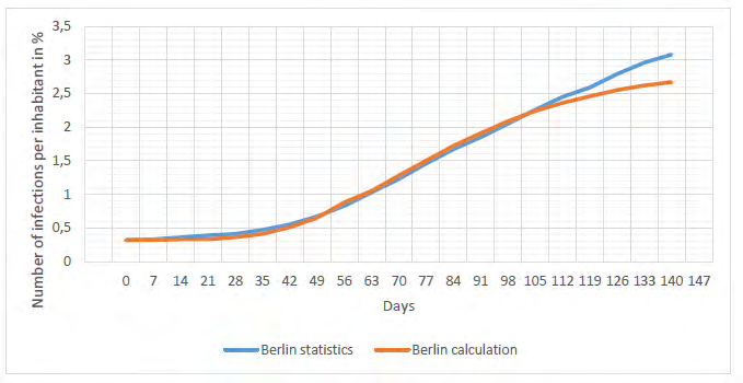
As a perimeter, Figure 4 shows a graph based on statistical data for Berlin [8]. In principle, the results of calculations and statistical data begin to deviate in the same way as for New York after about 90 days after the beginning of the second wave of the epidemic. The only reasonable explanation for this phenomenon is the assumption of the emergence of a third wave of the epidemic, associated with the spread of the virus strain found in the UK [9]. In this case, the calculation model needs some adjustment. The initial equation of the model under conditions of simultaneous spread of both types of virus can be written in the form:
1 (t t ) 1 100 {exp[ (1 e )] exp[ (1 e )]} t r r o k k i i Nr
λ λ δ λ λ $$ i = i _ {o} + \frac {1 0 0}{N r} * \left\{\exp \left[ \frac {k _ {r}}{\lambda} \left(1 - \mathrm {e} ^ {- \lambda t}\right) \right] + \delta * \exp \left[ \frac {k _ {1 r}}{\lambda} \left(1 - \mathrm {e} ^ {- \lambda * \left(t - t _ {1}\right)}\right) \right. \right. $$ (5) In which: 𝑘1𝑟 - is the transmission rate coefficient of the new virus strain and the time of the epidemic wave associated with the new coronavirus strain t1 - time of the beginning of the epidemic wave associated with the new coronavirus strain σ - Heaviside step function. σ = 1 when t ≥ 𝑡 1 and σ = 0 when t < 𝑡1 In this equation we additionally introduce a term describing the spread of a new wave of the epidemic, starting from the time t1. In the general case, considering that the intensity of the spread of the new strain may be different from the previous strain, the corresponding coefficient K1r is introduced. The coefficient λ according to the present model does not depend on the virus strain and is therefore taken as constant.
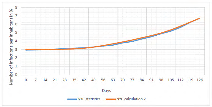
Figure 5 shows the comparison of results calculated by equation (5) with statistical data, taking into consideration that according to some data the new virus strain spreads more intensively, the value of Kr coefficient was slightly increased in calculations and we took K1r = 0,44 1/day.
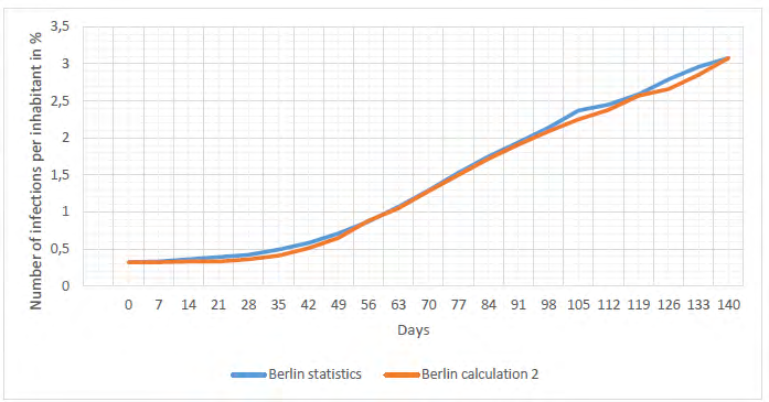
Similarly, we took into account that the third wave of epidemic also took place in Berlin. The corresponding data are presented on Figure 6. In the calculations by equation (5), the value of the coefficient K1r = 0.41 1/day was taken. The value of the coefficient λ was kept the same as in the previous calculations. Taking into account the third wave of the epidemic makes it possible to bring the calculated curve considerably closer to the real curve obtained from the analysis of statistical data. The choice of the start time of the third wave in calculations according to (5) should be particularly noted. Strictly speaking, the time of registration of the first patients with the mutated virus should be taken as the zero reference. However, in practice it is impossible to detect it. Therefore, it was conventionally assumed that the first manifestations of the new strain occur three weeks after the detection of the first patients. That means, the beginning of a new wave was taken as the time equal to 20 days before the first signs of a new increase in the intensity of the epidemic.
Discussion
As shown by comparing the results of calculations using the proposed model with statistical observations, the calculation errors are extremely small for both New York City and Berlin. We reached the same conclusion earlier for a number of Berlin districts [4]. If we compare the epidemic growth rate for both cities, the intensity of the spread of the first wave of infection in New York is incomparably higher than in Berlin, which can be explained by the fact that, when the first wave of the epidemic began, the New York City administration was considerably late in adopting restrictive measures. At the beginning of the new wave of the epidemic, due to the untimely introduction of quarantine measures, the epidemic was equally active in both cities. The high growth of the epidemic was due, in particular, to the lack of effective measures to control and limit the traffic between the cities and between the countries.
The good correspondence between the statistical and calculated data is sharply broken starting from December 2020, when there is a sharp increase in the epidemic in both cities. Apparently, the increase in the epidemic during this period of time could be explained by the increase in human contact between Christmas and New Year’s Eve. However, since the deviation from the calculated curve is observed long before Christmas we can accept with high probability that the emergence of a new strain of the virus is the cause of this increase in the intensity of the epidemic. A similar picture was revealed by us to a greater or lesser extent (the data have not been published, but are available to the authors of the work) when analyzing the growth of COVID 19 infections in Great Britain, Germany and a number of its cities (Munich, Dresden, Hamburg, Leipzig, etc.). Adjusting the model by introducing into it an additional term taking into account the appearance of the third epidemic wave allows for a fairly accurate calculation of the spread of infection for these conditions.
If we compare the increase in the number of infected in Berlin and New York to the initial number, then for the second wave of the epidemic these values practically coincide (Figure 7).
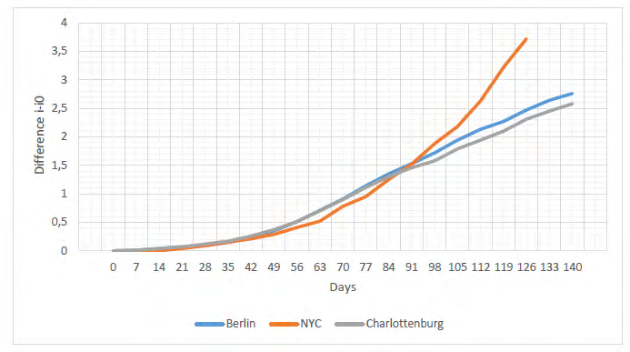
In order to exclude the influence of the previous wave, the difference between the current value of the number of infected people and their values at the time of the second wave is used. The same graph shows the development curve of the epidemic in one of Berlin’s districts, Charlottenburg. As can be seen from this figure, all three curves practically coincide up to a certain point in time. Only about 90 days after the beginning of this epidemic wave, the growth of the infection in New York became significantly higher than in Berlin and Charlottenburg. That means that the passage of the third wave of the epidemic for New York differs significantly from that of Berlin. At the same time, as we have already noted when discussing the graph in Figure 4, in Berlin there is also a slight increase in the number of infected people during this period of time, but it is noticeably more gradual. Apparently, the administration of New York was not fully prepared for the possibility of a sharp increase in the epidemic in December 2020 and January 2021. However, an unequivocal conclusion about the reasons for such an intense new growth of the epidemic can be made after special studies are performed.
The almost complete equivalence of the epidemic development schedules in Berlin and its separate district Charlottenburg testifies not only to the coincidence of their socio-demographic structure, but also to the same quarantine measures taken by the city administration. Thus, a detailed study of the growth patterns of the epidemic on the example of a district would provide reliable information applicable to larger sites. In addition, this correspondence of the data indicates that, in general, the process of spread of the infection is not subject to random but rather to quite deterministic patterns. Giving an overall assessment of the possibility of using an approximate model to calculate the intensity of virus epidemic spread, we can assume that this model can serve as a reliable tool for the operational analysis of the epidemic spread patterns. The successful use of this computational model implies the unambiguous choice of a single coefficient λ. In our previous work [4], we analyzed the influence of some factors on the value of this coefficient. However, since this coefficient is determined by the intensity of virus transmission as a result of contacts between people, the most important goal of further improvement of this model can be considered the establishment of a relationship between this coefficient and the characteristic behavioral characteristics of different population groups. Attempts are currently being made to link the risks of viral disease and transmission to a psychological characteristic, which has been named (BIS) [9]. In addition to these behavioral characteristics, socio-demographic characteristics of both cities and large urban areas are also important.
These crucial questions have been poorly studied so far and should be considered paramount in understanding the mechanisms of epidemic development. A detailed study of the patterns of epidemic development and an analysis of the criteria on which the intensity of this process depends for different typical conditions will make it possible to predict more reliably the risks of repeated waves of intensive growth of morbidity. At the same time, taking into account that preventing an epidemic is a much easier task than reducing the number of infected persons at high levels, forecasting the possible onset of an epidemic and developing specific targeted measures to sharply reduce the spread of infection among selected population groups will prevent the most negative consequences. These are both related directly to the growth of the disease, to reducing the risk of a sharp economic decline and to a considerable decrease in the population’s income.
Conclusions
The Conclusions for the results analyzed in the sections above are:
- The proposed simple analytical model shows quite satisfactory correspondence between the calculated results and the statistical observations on the intensity of spread of COVID 19 epidemic.
- The ease of use of the calculation methodology and the sufficient accuracy of the calculations will allow its use by the administrative authorities as an additional operational tool to control the possibility of repeated waves of epidemics in their earliest stages.
- Further improvement of the model is planned, first of all in the direction of determining the links between the intensity of transmission of the infection which is the coefficient λ with psychological and behavioral characteristics of different socio- demographic groups of the population and quarantine conditions. This will make it possible to use the model not only for calculations of epidemic growth, but also for operational forecasting.
- The analysis of the passage of different epidemic waves in New York and Berlin allows us to draw some preliminary conclusions concerning the efficiency of the control of the epidemic in both cities.
- The coincidence of the epidemic development schedules for Berlin and Charlottenburg allows us to conclude about the deterministic nature of the spread of the infection. Thus, there is an opportunity to study in detail the growth patterns of the epidemic in large cities on the basis of studies carried out for analogous small areas or compact settlements.
References
-
Below D, Mairanowski J, Mairanowski F (2021) Analysis of the intensity of the COVID-19 epidemic in Berlin towards an universal prognostic relationship. medRxiv pp: 1-16.
-
Below D, Mairanowski J, Mairanowski F (2020) Checking the calculation model for the coronavirus epidemic in Berlin. The first steps towards predicting the spread of the epidemic. medRxiv pp: 1-16.
-
Below D, Mairanowski F (2020) Prediction of the coronavirus epidemic prevalence in quarantine conditions based on an approximate calculation model. medRxiv pp: 1-12.
-
Dobkin J, Diaz C, Gotterer CZ (2021) Coronavirus Statistics: Tracking the Epidemic In New York. Gothamist.
-
(2020) Verordnung über erforderliche Maßnahmen zur Eindämmung der Ausbreitung des neuartigen Coronavirus SARS-CoV-2 in Berlin vom 17.
-
Maier BH, Gebske J, Schluter A (2021) Corona-Grafiken- Berliner Ampel-Das sind die aktuellen Fallzahlen in Berlin und Brandenburg. Rbb24.
-
(2021) Der Regierende Bürgermeister von Berlin- Senatskanzlei Informationen zum Coronavirus (Covid-19).
-
ECDC (2020) Rapid increase of a SARS-CoV-2 variant with multiple spike protein mutations observed in the United Kingdom. European Centre for Disease Prevention and Control, Stockholm pp: 1-13.
-
Bacon AM, Corr PJ (2020) Behavioral Immune System Responses to Coronavirus: A Reinforcement Sensitivity Theory Explanation of Conformity, Warmth toward Others and Attitudes toward Lockdown. Front Psychol 11: 566237.
- Intersecting Epidemics and Climate Vulnerabilities in Conflict- Driven Displacement: Epidemiology, Systemic Challenges, and One Health Gaps in South Sudan
- Advancing Domestic Health Financing for Community Health System Sustainability in South Sudan: The Boma Health Initiative Model (2025–2035)
- Prevalence and Correlates of Post-Exposure Prophylaxis Uptake among Men Who Have Sex with Men in Kisumu County, Kenya
- Medical, Ethical, and Legal Conflicts Surrounding Euthanasia in Argentina. Its Global Implications
- Knowledge and Attitude on Menstrual Hygiene among Adolescent Girls Studying in Secondary Level in Public Schools of Chitwan District, Nepal
- Biological Efficacy of an Adulticide Mixture (clothianidin + deltamethrin) as an Indoor Residual Spray against Adult Anopheles flavirostris in Palawan, the Philippines