Pati-Salam Model in Curved Space-Time from Square Root Lorentz Manifold
There is a U U (4' 4 ) × ( ) -bundle on four-dimensional square root Lorentz manifold. Then a Pati-Salam model in curved space-time (Lagrangian) and a gravity theory (Lagrangian) are constructed on square root Lorentz manifold based on self-parallel transportation principle. An explicit formulation of Sheaf quantization on this square root Lorentz manifold is shown. Sheaf quantization is based on superposition principle and construct a linear Sheaf space in curved space-time. The transition amplitude in path integral quantization is given which is consistent with Sheaf quantization. All particles and fields in Standard Model (SM) of particle physics and Einstein gravity are found in square root metric and the connections of bundle. The interactions between particles/fields are described by Lagrangian explicitly. There are few new physics in this model. The gravity theory is Einstein-Cartan kind with torsion. There are new particles, right handed neutrinos, dark photon, Fiona, c X ± and 01212 * * YYYYY ,,,, .
Introduction
Four-dimensional pseudo-Riemann geometry with signature $(-,+,+,+)$, Lorentz manifold, is the geometry background of the general relativity, space-time is described by the metric, and the gravitational field is described as the curve of space-time. In general relativity, the geodesic equation describes the trajectories of free particles, and the Einstein equation determines how matter curves space-time. At the last life time of Einstein, he attempted to establish a new geometry unifying electromagnetic interaction and gravity. This idea was developed by Weil into the early idea of gauge invariance and by the Kaluza and Klein into the idea of extra dimensions.
Later, the Yang-Mills theory [1] was confirmed. Yang-Mills theory takes gauge invariance as its basic principle and to be the theoretical framework of electromagnetic, weak and strong interaction in Standard Model (SM) of particle physics [2, 3, 4, 5, 6, 7]. The Yang-Mills theory is the theoretical framework of SM and has a good correspondence with the complex structure group G fiber bundle theory [8]. General relativity can actually be rewritten in the framework of fiber bundle theory also, except that the G structure group of general relativity is real, and the corresponding fiber bundles are the tangent and cotangent bundles. Another way to build unified field theory is introducing extra dimensions to give all fields their geometric positions. And lots of attempts in extra dimension were made. Is it possible to fuse the tangent (cotangent) bundle of general relativity with the complex structure group G-bundle of Yang-Mills theory?
Inspired by the Dirac’s way of finding his equation and
spinors through making square root of the Klein-Gordon
equation, we researched the four-dimensional square root
Lorentz manifold, which similar with the papers in Clifford
algebra or Clifford bundle [9, 10, 11, 12, 13, 14, 15, 16, 17, 18, 19, 20, 21, 22, 23, 24, 25, 26, 27, 28, 29, 30, 31, 32, 33, 34, 35, 36, 37, 38, 39, 40, 41, 42, 43, 44, 45, 46, 47, 48, 49, 50, 51, 52], spin-gauge theory in
Riemann-Cartan space-time [53, 54], sedenion [55] and
Einstein-Cartan theory [56, 57, 58] etc. Four-dimensional
square root Lorentz manifold has extra
$$ U \left(4 ^ {\prime}\right) \times U (4) $$
principal bundle than Lorentz manifold. Two Lagrangians
based on four-dimension square root Lorentz manifold are
constructed which describe a
( ) ( ) ( ) 4' 4 4 L R U U U × × Pati-
Salam model in curved space-time and a gravity theory,
respectively. In the Pati-Salam model [59], the
( ) '4 SU is
color group with “lepton number as the fourth color”, and the ( ) ( ) 4 4 L R SU SU × is chiral flavor group. The gravity theory is Einstein kind with torsion. We realize an explicit formulation of Sheaf quantization [60, 61, 62, 63, 64, 65, 66, 67, 68, 69, 70, 71, 72, 73, 74, 75, 76] scheme which consistent with path integral quantization. The particles spectrum on this model is analyzed.
Geometry and Lagrangian
The notations are introduced here. , , , a b c d represent frame indices and , , , a b c d are equal to 0,1,2,3 . , , , v µ ρ σ represent coordinates indices and , , , v µ ρ σ are equal to 0,1,2,3 . α represent group indices with α equals to
0,1,....,15. , , , , i j k l m are equal to 1,2,3,4 . C is quarks color and equals to ( ) , , 1,2,3 R G B . k is Sheaf space index. Repeated indices are summed by default.
The pseudo-Riemann manifold is described by a metric $$ g (x) = - g _ {\mu \nu} (x) d x ^ {\mu} d x ^ {\nu}, \tag {1} $$ where the metric is symmetric $$ g _ {\mu \nu} (x) = g _ {\nu \mu} (x), \tag {2} $$ $$ \text {a n d} \left\{x \mid x = \left(x ^ {\mu}\right) = \left(t, \vec {x}\right) \right\} i $$
is a four-dimensional topological
space. Here we discuss the four-dimensional pseudo-
Riemann manifold with signature(
) , , ,
−+ + + , Lorentz
manifold. And it can be described by orthonormal frame
(vierbein) formalism as ( ) ( ) ( ) 1 , ab a b g x x x η θ θ − = − (3) where ( ) 1, 1, 1, 1 . ab diag η = −−− orthonormal frames describe gravitational field (Figure 1).
$$ \theta_ {a} (x) = \theta_ {a} ^ {\mu} (x) \frac {\partial}{\partial x ^ {\mu}}. $$ ( ) ( ) . a a x x x
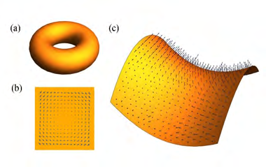
(a) general relativity (b) Yang-Mills theory and (c) square
root metric. (a) Geometry background of general relativity
is pseudo-Riemann geometry, which is a smooth curved
manifold. (b) Geometry background of Yang-Mills theory
is complex G-bundle with flat base manifold, G is the
gauge group of Yang-Mills theory. (c) Square root metric
geometry in four-dimension has everything of pseudo-
Riemann geometry and extra
$$ U \left(4 ^ {\prime}\right) \times U (4) - b u n d l e. $$ The definition of gamma matrices is $$ \gamma^ {a} \gamma^ {b} + \gamma^ {b} \gamma^ {a} = 2 \eta^ {a b} I _ {4 \times 4}. \tag {4} $$ The Hermiticity conditions for gamma matrices are $$ \gamma^ {a} \gamma^ {b \dagger} + \gamma^ {b \dagger} \gamma^ {a} = 2 I ^ {a b} I _ {4 \times 4}, \tag {5} $$ where ab I is ( ) 1,1,1,1 diag . We define $$ l = i \gamma_ {i k} ^ {0} (x) \gamma_ {k j} ^ {a} (x) e _ {j} ^ {\dagger} \otimes e _ {j} \theta_ {a} (x), \tag {6} $$ $$ \tilde {l} = i \gamma_ {i k} ^ {a} (x) \gamma_ {k j} ^ {0} (x) e _ {j} ^ {\dagger} \otimes e _ {i} \theta_ {a} (x), \tag {7} $$ where ie are the orthogonal bases expanding four-dimension complex space 4 ≤. The orthogonal bases of 4 ≤ satisfy $$ t r \left(e _ {j} ^ {\dagger} \otimes e _ {i}\right) = e _ {i} e _ {j} ^ {\dagger} = \delta_ {i j}. \tag {8} $$ One simple choice of ie is $$ e _ {1} = \left(e ^ {i \theta_ {1}}, 0, 0, 0\right), e _ {2} = \left(0, e ^ {i \theta_ {2}}, 0, 0\right), \tag {9} $$ ( ) ( ) 3 4 3 4 0,0, ,0 , 0,0,0, . i i e e e e θ θ = = (10) After using † 0 0 a a γ γ γ γ = , we find that $$g^{-1}(x) = \frac{1}{4} \text{tr} \left[ \bar{l}(x) l(x) \right]. \tag{11}$$
Then $l(x)$ and $\bar{l}(x)$ are the square root of metrics in some sense. The representation freedom of $\gamma_{ij}^{a}(x)$ can be shown as
$$\gamma_{ik}^{0}(x) \gamma_{kj}^{a}(x) = \psi_{ik}^{\dagger}(x) \gamma_{kl}^{0} \gamma_{lm}^{a} \psi_{mj}(x) = \bar{\psi}_{i}(x) \gamma^{a} \psi_{j}(x),$$
$$\gamma_{ik}^{a}(x) \gamma_{kj}^{0}(x) = \psi_{ik}^{\dagger}(x) \gamma_{kl}^{a} \gamma_{lm}^{0} \psi_{mj}(x) = \bar{\psi}_{i}(x) \gamma^{a \dagger} \psi_{j}(x),$$
where $\psi_{i}$ are the Dirac fermions field with flavor related index $i$ equals to 1,2,3,4. And
$$\bar{\psi}_{i}(x) = \psi_{i}^{\dagger}(x) \gamma^{0}, \psi(x) \in U(4)$$
is $4 \times 4$ matrix. So, the square root metrics are defined as follow
$$l(x) = i \bar{\psi}_{i}(x) \gamma^{a} \psi_{j}(x) e_{j}^{\dagger} \otimes e_{i} \theta_{a}(x), \tag{12}$$
$$\bar{l}(x) = i \bar{\psi}_{i}(x) \gamma^{a \dagger} \psi_{j}(x) e_{j}^{\dagger} \otimes e_{i} \theta_{a}(x). \tag{13}$$
The square root Lorentz manifold is described by square root metric (12), (13). Direct calculations show that the definition (12) and (13) satisfy (11) and
$$l^{\dagger}(x) = -l(x), \bar{l}^{\dagger}(x) = -\bar{l}(x).$$
The coefficients of the affine connections on coordinates, coefficients of spin connections on orthonormal frame [77] and gauge fields on the $U(4) \times U(4)$-bundle are defined as follows
$$\nabla_{\mu} \partial_{v} = \Gamma_{\nu\mu}^{p}(x) \partial_{p}, \tag{14}$$
$$\nabla_{\mu} \theta_{a}(x) = \Gamma_{\nu\mu}^{b}(x) \theta_{h}(x), \tag{15}$$
$$\nabla_{\mu} \left( \gamma^{0} \gamma^{a} \right) = i \left[ V_{\mu}(x) \gamma^{0} \gamma^{a} - \gamma^{0} \gamma^{a} V_{\mu}(x) \right], \tag{16}$$
$$\nabla_{\mu} e_{i} = i W_{\mu j}(x) e_{j}^{\dagger}. \tag{17}$$
A relation between coefficients of the affine connections on coordinates and coefficients of spin connections on orthonormal frame can be easily found
$$\Gamma_{a\mu}^{b}(x) \theta_{b}^{a}(x) = \partial_{\mu} \theta_{a}^{b}(x) + \theta_{a}^{b}(x) \Gamma_{v\mu}^{p}(x).$$
If the covariant derivative is compatible with metric,
$$\nabla g(x) = 0,$$
then
$$\Gamma_{ab\mu} = -\Gamma_{ba\mu}.$$
The gauge fields on the $U(4) \times U(4)$-bundle are Hermitian
$$V_{ij}^{a}(x) = V_{ij}(x), W_{ij}^{b}(x) = W_{ij}(x).$$
The uniqueness of definition of gauge fields is originated from restriction (4), (5) and (8). The equation as follow can be derived from (16)
$$\nabla_{\mu} \left( \gamma^{a} \gamma^{0} \right) = i \left[ \bar{\nabla}_{\mu}(x) \gamma^{a} \gamma^{0} - \gamma^{a} \gamma^{0} \bar{\nabla}_{\mu}(x) \right], \tag{18}$$
where we write
$$\bar{\nabla}_{\mu}(x) = \gamma^{0} V \gamma^{0}.$$
The gauge field $V_{\mu}(x)$ and $W_{\mu j}(x)$ can be decomposed by the generators of the $U(4)$ group
$$V_{\mu}(x) = V_{\mu}^{a}(x) T^{\alpha}, \tag{19}$$
$$W_{\mu j}(x) = W_{\mu}^{a}(x) T_{ij}^{\alpha}, \tag{20}$$
where $\alpha$ is equals to 0,1,2,...15. There are Hermitian gauge bosons fields
$$V_{\mu}^{\alpha \dagger}(x) = V_{\mu}^{a}(x), W_{\mu}^{\alpha \dagger}(x) = W_{\mu}^{a}(x).$$
The $T^{\alpha}$ are the generators of $U(4)$ and an explicit one can be seen in appendix. An equation is constructed which satisfying the $U(4^{\prime}) \times U(4)$ gauge invariant, locally Lorentz invariant and generally covariant principles
$$\text{tr} \nabla[l(x)] = 0. \tag{21}$$
This equation originated from generalized self-parallel transportation principle. Eliminating index $x$, the explicit formula of equation (21) is
$$\left[ i \partial_{\mu} \bar{\psi}_{i} - \bar{\psi}_{i} \bar{V}_{\mu} + W_{\mu j} \bar{\psi}_{j} \right] \gamma^{a} \psi_{i} + \bar{\psi}_{i} \gamma^{a}$$
$$\left[ i \partial_{\mu} \psi_{i} + V_{\mu} \psi_{i} - \psi_{j} W_{\mu j} \right] \psi_{i} \gamma^{b} \psi_{i} \Gamma_{a\mu}^{\alpha} \theta_{a}^{\alpha}. \tag{22}$$
The last term in Lagrangian (22) is Yukawa coupling term $\psi_{i} \phi \psi_{i}$ and the scalar (Higgs) field is gamma matrix valued and originated from gravitational field.
$$\phi = \frac{i}{2} \gamma^{b} \Gamma_{a\mu}^{\alpha} \theta_{a}^{\alpha}. \tag{23}$$
Then, the Lagrangian (22) describes $U(4') \times U(4)$ Yang-Mills theory in curved space-time (Figure 1). The Lagrangian (22) has relation with (21)
$$\text{tr} \nabla [l(x)] = \mathcal{L} - \mathcal{L}'.$$ (24)
If equation (21) being satisfied, the Lagrangian (22) is Hermitian
$$\mathcal{L} = \mathcal{L}'.$$ (25)
So, the unitary principle of quantum field theory (25) consistent with generalized self-parallel transportation principle (21). The equations of motion for the Lagrangian (22) are
$$\gamma^a \left( i \partial_\mu \psi_i + V_\mu \psi_j - \psi_j W_{\mu j} \right) \theta_a^a + \frac{i}{2} \gamma^b \psi_i \Gamma_a^b \theta_a^a = 0,$$ (26)
and this equation’s conjugate transpose. We point out that (21) is density matrix version of (26). The effective equation of motion of (26) has signature (1, -1, -1, -1). For example, the massless Dirac equation in curved space-time of this model is
$$i \gamma^a \theta_a^a \partial_\mu \psi_i = 0.$$ (27)
The square of equation (27) is massless Klein-Gordon equation in curved space-time
$$\eta^{ab} \theta_a^a \theta_b^a \partial_\mu \partial_v \psi_i = 0.$$ (28)
The signature of equation (28) is $(1, -1, -1, -1)$ and consistent with special relativity. Then, a Lagrangian (22) which describes the $U(4') \times U(4)$ Yang-Mills theory in curved space-time is all other fields (except Higgs field) dynamical background which satisfies the characteristic of the gravitational field in our real world.
Lagrangian (22) is $U(4') \times U(4)$ gauge invariant, locally Lorentz invariant and generally covariant. So, Lagrangian (22) is demanded invariant under the transformations
$$\psi_i = \tilde{U} \psi_j U_{ji},$$
$$\gamma^a = \tilde{U} \gamma^b \tilde{U}^\dagger \Lambda_b^a,$$ (29)
$$\theta_a^a = \Lambda_b^a \theta_b^a,$$
Then, the transformation rules have to be derived as follows
$$V_\mu = \tilde{U} V_\mu \tilde{U}^\dagger - \left( \partial_\mu \tilde{U} \right) \tilde{U}^\dagger,$$ (30)
$$V_\mu = U_{ki} W_\mu U_{ij} + U_{ki} \left( \partial_\mu W_{ij} \right),$$ (31)
$$\Gamma_{b\mu}^b = \Lambda_a^a \Gamma_{c\mu}^d \Lambda_d^b - \Lambda_a^a \partial_\mu \Lambda_c^b,$$ (32)
where the transformation matrices satisfy
$$\tilde{U} \tilde{U}^\dagger = I, U_{ji} U_{ji}^* = \delta_{ik}, \Lambda_a^b \Lambda_b^c = \delta_a^c.$$
Then the transformation elements
$$\tilde{U} \in U(4'),$$
$$\left( U_{ij} \right) \in U(4),$$
$$\Lambda_b^a \in O(1,3),$$
and $U(4)$ is color group, $U(4)$ is flavor group, $O(1,3)$ is locally Lorentz group. Then we complete the proof of the Lagrangian (22) is $U(4') \times U(4)$ gauge invariant, locally Lorentz invariant and generally covariant.
The gauge field strength tensors and curvature tensor are defined as follows
$$H_{\mu v} = \partial_\mu V_\mu - \partial_v V_\mu - i V_\mu V_v,$$
$$F_{\mu vj} = \partial_\mu W_{vj} - \partial_v W_{vj} - i W_{\mu k} W_{vkj},$$
$$R_a^b_{b\mu} = \partial_\mu \Gamma_a^b_{b\mu} - \partial_v \Gamma_a^b_{b\mu} + \Gamma_b^c \Gamma_c^a - \Gamma_c^b \Gamma_c^a.$$
If the covariant derivative is compatible with metric, the curvature tensor satisfies
$$R_{ab\mu\nu} = -R_{bau\nu}.$$
The gauge fields strengths on the $U(4') \times U(4)$-bundle match the Hermiticity conditions
$$H^\dagger_{\mu v} = H_{\mu v}, F_{\mu vj}^* = F_{\mu vj}.$$
The gauge field strength can be decomposed by the $U(4)$ generators
$$H_{\mu v} = H_{\mu v}^a T_a^a, F_{\mu vj} = F_{\mu v}^a T_{ij}^a.$$
After the torsion being defined
$$T_{vp}^a = 2 \Gamma_a^a_{[vp]},$$ (33)
we have the Ricci identity and Bianchi identity [78] on this geometry structure as follows
$$\partial_{\mu} H_{vp} = H_{[vp} V_\rho] - V_{\mu} H_{vp},$$ (34)
$$\partial_{\mu} F_{vp} = F_{[vp] k} W_\rho^k - W_{\mu k} F_{vp} k_j,$$ (35)
$$T_a^a_{\rho} T_{vp} = R_a^a_{\rho} + \nabla_{\rho} T_{a\nu}.$$ (36)
$$ \nabla_ {[ \rho} R _ {| b | \mu \nu ]} ^ {a} = R _ {b \sigma [ \rho} ^ {a} T _ {\mu \nu ]}. \tag {37} $$ There is Yang-Mills Lagrangian for gauge bosons in this model $$ \mathcal {L} _ {Y} = \frac {- 1}{2} \boldsymbol {t r} \left(H ^ {\mu \nu} H _ {\mu \nu}\right) - \frac {- \zeta}{2} F _ {i j} ^ {\mu \nu} F _ {\mu \nu j i}, $$ (38) where R ζ ∈ is constant.
For the gravity, the Einstein-Hilbert action in Lorentz manifold be showed as follow $$ S = \int \omega R, \tag {39} $$ where is the Ricci scalar curvature in Lorentz manifold, ω is volume form $$ \omega = \sqrt {- g _ {v}} d x ^ {0} \wedge d x ^ {1} \wedge d x ^ {2} \wedge d x ^ {3} $$ and $$ g _ {v} = \det \left(g _ {\mu v} (x)\right). $$ In this geometry framework, the equations can be derived as follows * [ ] 1( 2 $$ \nabla_ {[ \mu} \nabla_ {\nu ]} l = \frac {- 1}{2} \left(\psi_ {i} \gamma^ {a} \psi_ {k} F _ {\mu \nu k j} - F _ {\mu \nu k i} ^ {*} \bar {\psi} _ {k} \gamma^ {a} \psi_ {j} + \bar {\psi} _ {i} \tilde {H} _ {\mu \nu} \gamma^ {a} \psi_ {j}\right) $$ $$ - \bar {\psi} _ {i} \gamma^ {a} H _ {\mu \nu} \psi_ {j} + \frac {i}{2} \bar {\psi} _ {i} \gamma^ {b} \psi_ {j} R _ {b \mu \nu} ^ {a}) e _ {j} ^ {\dagger} \otimes e _ {i} \theta^ {a}, \tag {40} $$ † ) , 2 † * † † [ ] 1( 2 $$ \nabla_ {[ \mu} \nabla_ {\nu ]} \tilde {l} = \frac {- 1}{2} \left(\psi_ {i} \gamma^ {a ^ {\dagger}} \psi_ {k} F _ {\mu \nu k j} - F _ {\mu \nu k i} ^ {*} \bar {\psi} _ {k} \gamma^ {a ^ {\dagger}} \psi_ {j} + \bar {\psi} _ {i} \tilde {H} _ {\mu \nu} \gamma^ {a ^ {\dagger}} \psi_ {j}\right) $$ $$ - \bar {\psi} _ {i} \gamma^ {a \dagger} H _ {\mu \nu} \psi_ {j} + \frac {i}{2} \bar {\psi} _ {i} \gamma^ {b \dagger} \psi_ {j} R _ {b \mu \nu} ^ {a}) e _ {j} ^ {\dagger} \otimes e _ {i} \theta^ {a}, \tag {41} $$
where we write † † † ) , 2 $$ \tilde {H} _ {\mu \nu} = \gamma^ {0} H _ {\mu \nu} \gamma^ {0}. $$ We define $$ \nabla^ {2} = \nabla_ {[ \mu} \nabla_ {\nu ]} d x ^ {\mu} \wedge d x ^ {\nu}, $$
the equation of a gravity theory is constructed $$ \boldsymbol {t r} \nabla^ {2} \left[ \tilde {l} (x) l (x) \right] = 0. \tag {42} $$ This equation (42) is obviously (4 ) ') (4 U U × gauge invariant, locally Lorentz invariant and generally covariant. The explicit formula of equation (42) is ( ) † † † † ( abij a b b a i i j i R i F ψ ψ ψ γ γ γ γ ψ = − $$ - \psi_ {i} ^ {\dagger} H _ {a b} \left(\gamma^ {a} \gamma^ {b} - \gamma^ {b \dagger} \gamma^ {a \dagger}\right) \psi_ {i}, \tag {43} $$ where we use the notations as follow, $$ \partial_ {\mu} d x ^ {\nu} \otimes d x ^ {\rho} \partial_ {\sigma} = \delta_ {\mu} ^ {\nu} \delta_ {\sigma} ^ {\rho}, $$ $$ d x ^ {\mu} \otimes d x ^ {\nu} \partial_ {\rho} \partial_ {\sigma} = \delta_ {\rho} ^ {\nu} \delta_ {\sigma} ^ {\mu}, $$ $$ F _ {a b i j} = F _ {a b i j} \theta_ {a} ^ {u} \theta_ {b} ^ {v}, $$ $$ H _ {a b} = H _ {\mu \nu} \theta_ {a} ^ {u} \theta_ {b} ^ {v}. $$ So, we define a
$$ U \left(4 ^ {\prime}\right) \times U (4) $$
gauge invariant, locally Lorentz
invariant, generally covariant Lagrangian ( ) † † † † abij a b b a g i i j i † † † ( R i F ψ ψ ψ γ γ γ γ ψ $$ = R \psi_ {i} ^ {\dagger} \psi_ {i} - i \left(F ^ {a b i j} \psi_ {j} ^ {\dagger} \left(\gamma^ {a} \gamma^ {b} - \gamma\right\right) $$ Λ (44) ( ) a b b a i ab i .
i H
ψ γ γ γ γ ψ + −
The Lagrangian (44) is Hermitian
$$ \mathcal {L} _ {g} = \mathcal {L} _ {g} ^ {\dagger}. \tag {45} $$
The † i i Rψ ψ in Lagrangian (44) gives us the Einstein-Hilbert action. The equation (43) and the Einstein tensor can be derived from the Lagrangian (44). The gravity theory in this model is Einstein-Cartan kind with torsion.
Sheaf Quantization and Path Integral Quantization
The entities ( ) l x and ( ) l x are two sections of the two bundles, respectively, where these two bundles are dual to each other. Further, the Sheaf valued entities ( ) ˆl x and ( ) l x are superposition of sections ( ) l x and ( ) l x (Figure 2).
$$ \hat {l} (x) = \sum_ {\kappa} \eta_ {\kappa} (x) \left| \kappa , x \right\rangle \langle \kappa , x \mid l _ {\kappa} (x), \tag {46} $$ $$ \hat {\tilde {l}} (x) = \sum_ {\kappa} \eta_ {\kappa} (x) | \kappa , x \rangle \langle \kappa , x | \tilde {l} _ {\kappa} (x), \tag {47} $$
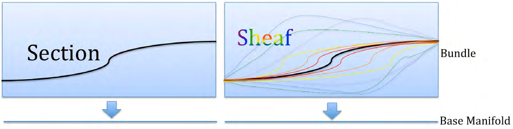
where ( ) [ ] 0,1 x κ η ∈ are probability of corresponding section ( ) l x κ and ( ), l x κ κ is Sheaf space index and evaluated in an abelian group. The density matrix corresponds to ( ) ˆl x and ( ) l x is $$ \rho (x) = \sum_ {\kappa} \eta_ {\kappa} (x) \left| \kappa , x \right\rangle \langle \kappa , x |. \tag {48} $$ We have orthogonal bases in Sheaf space. The orthogonal bases in Sheaf space satisfy probability complete formulas $$ \left\langle \kappa , x \mid \kappa^ {\prime}, x ^ {\prime} \right\rangle = \delta \left(x - x ^ {\prime}\right) \delta \left(\kappa - \kappa^ {\prime}\right). \tag {49} $$ $$ \operatorname {t r} \rho (x) = \sum_ {\hat {\mathrm {e}}} \eta_ {\kappa} (x) = 1. \tag {50} $$ ( ) ( ) In mathematics, a Sheaf is a collection of sections, the index κ of each section correspond to an abelian group element. In physics, the Sheaf spaces ( ) Sh x and ±( ) Sh x are expanded by all possible sections ( ) l x and ( ) l x of the two bundles, respectively. The ( ) Sh x and ±( ) Sh x are linear spaces, which means, for example, any two entities ( ) 1ˆl x and ( ) 2ˆl x in ( ) Sh x , there is an entity ( ) ˆl x in ( ) Sh x equals to the mixing of the two entities ˆ ˆ ˆ ( ) ( ) ( ) ( ) ( ) , l x x l x x l x $$ ) = \eta_ {1} (x) \hat {l} _ {1} (x) + \eta_ {2} () $$
1 1 2 2 ˆ ˆ
( ) ( ) ( )
, ;
l x l x Sh x ∈
(51)
1 2 ˆ
( ) ( ) , l x Sh x ⇒ ∈
where the probability of each section ( ) ( ) [ ] 1 2 , 0,1 x x η η ∈ and $$ \eta_ {1} (x) + \eta_ {2} (x) = 1. $$ The Sheaf spaces ( ) Sh x and ±( ) Sh x are dual to each other. We call it Sheaf quantization which switching study objects from single section to all possible sections of the bundle. The equation (50) derives to equation of motion for density matrix $$ d \left(\boldsymbol {t r} \rho (x)\right) = \boldsymbol {t r} \left(d \rho (x)\right) = 0, \tag {52} $$ where d is exterior differential derivative. The equations of motion for entities ( ) ˆl x and ( ) l x in Sheaf quantization method are $$ \boldsymbol {t r} \nabla \left[ \hat {l} (x) \right] = 0, \boldsymbol {t r} \left[ \hat {\hat {l}} (x) \hat {l} (x) \right] = 0. \tag {53} $$ The corresponding total Lagrangian density is , , , ˆ g Y g g κ κ κ κ = + + ∑ Λ Λ Λ Λ (54) where g and g are Lagrangian multipliers with , . g g ∈ For pure state $$ \rho (x) = \left| \Psi (x) \Psi (x) \right|, \tag {55} $$ $$ \left| \Psi (x) \right\rangle = \sum_ {\kappa} \alpha_ {\kappa} (x) | \kappa \rangle , \tag {56} $$ where the ( ) x Ψ is the quantum state of quantum field theory. The transition amplitude can be defined through path integral formula , 0 t t ,t ρ ρ ρ ρ Λ (57) ˆ , , , , i t x t x D t x e t x ω κ κ κ α κ α ( ) ( ) ( ) ( ) ( ) $$ ) = \int_ {t ^ {\prime} \in \left(t _ {0}, t\right)} D \kappa \left(t ^ {\prime}, \vec {x}\right) e ^ {i \omega \hat {\mathcal {L}} \left[ \kappa \left(t, \vec {x}\right) \right]} d $$ ∈ ′
0 where ω is volume form.
Particles Spectrum
µ V α and µ
W α (α is equals to 0,1 ,
bosons fields. The interactions related with the gauge bosons
fields µ
W α always preserves the possibility of chiral symmetry
breaking in the Lagrangian (54) such that the gauge group
can be decomposed to
$$ U \left(4 ^ {\prime}\right) \times U \left(4\right) _ {L} \times U \left(4\right) _ {R}, \text {w h e r e} U \left(4 ^ {\prime}\right) $$
is color group and
( ) ( ) 4 4 L R U U ×
is chiral flavor group. The
0 µ
V is dark photon and
0 µ
W is Fiona particle.
0 µ V and 0 µ W are related with ( ) 1 U ′ and ( ) 1 U
gauge group in
( ) 4 U ′ and ( ) 4 U
, respectively. The left-over gauge group is a Pati-Salam gauge
group ( ) ( ) ( ) 4 4 4 L R SU SU SU × × ′
( ) 4 SU
′ gauge group can be decomposed as follow $$ U \left(4 ^ {\prime}\right) = S U \left(3 ^ {\prime}\right) \oplus U \left(1 ^ {\prime}\right) + U _ {X ^ {+}} + U _ {X ^ {-}}. \tag {58} $$
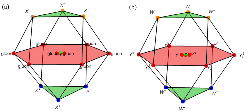
adjoint representation is
$$ 1 5 = 8 \otimes 1 + 3 + 3 ^ {*}. \tag {a} $$
The wight diagram of V α
µ which contained gauge bosons
are gluons, photon and
$$ \left[ X _ {v ^ {0}} ^ {\mu} ^ {\pm C}. \right] $$
(b) The wight diagram of W α µ
related gauge bosons are
$$ Y ^ {0}, Y ^ {1}, Y ^ {2}, Y _ {*} ^ {1}, Y _ {*} ^ {2} \mathrm {a n d} W ^ {\pm}, Z. $$ The ( ) 3 SU ′ is the gauge group of quantum chramodynamics (QCD) and the corresponding gauge bosons µ V α (α is equals to 1, 2
$$ X ^ {+ C} \mathrm {a n d} X ^ {- C} \mathrm {a r e} 1 / 3 \mathrm {a n d} $$
−1/3, respectively. The chiral gauge group
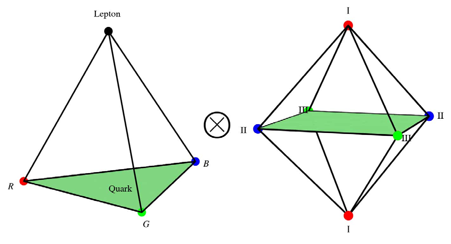
( ) , 4 L R SU can be
decomposed as (Figure 4).
$$ S U \left(4\right) _ {L, R} = S U \left(3\right) _ {Y} \oplus U \left(1\right) _ {Z} + U _ {W ^ {+}} + U _ {W ^ {-}}, \tag {60} $$ and related gauge bosons µ V α (with α equals to1, 2,
9 10 11 12 W W iW W iW (61)
µ µ µ µ µ
13 14, W iW
= ± µ µ $$ Z _ {\mu} = W _ {\mu} ^ {1 5}. \tag {62} $$
The left over gauge bosons are 0 1 2 1 2 * * , , , , Y Y Y Y Y with 0 electric charge. The gauge bosons 1 2 1 2 * * , , , Y Y Y Y transport non-SM flavor changing neutral currents (FCNCs) and (63) $$ \text {The} X ^ {\pm C} \text {and} Y ^ {1}, Y ^ {2}, Y _ {*} ^ {1}, Y _ {*} ^ {2} $$
Y Y must be super heavy from the
restrictions of experimental data.
The fermionic fields
i
ψ transfer as the
$$ U \left(4 ^ {\prime}\right) \times U (4) $$
fundamental representation according to (29). So, fermions
are filled into the
( ) 4 SU fundamental representation ⊗ 4 6
naturally. The fundamental representation 4 corresponds to
3 colors and 1 lepton and leads us reobtain “Lepton number as the fourth color” [59]. The fundamental representation 6 corresponds to 6 flavors of quarks and leptons. The weight diagram coordinates in Chevalley basis of representation 6 (see in Table 1) have good correspondence with the quark quantum number [80]. The antifermions be filled into the representation ⊗ 6 4 similarly. The weight diagram of fermions is shown in Figure 4. Both left-handed and right- handed fermions for all quarks and leptons are existed. Especially, the existence of right-handed neutrinos is predicted. This is compatible with experimental results [81] and the well know Seesaw mechanism [82, 83, 84, 85, 86]. The 2 zI being used in Table I are not no reasons because we have the Gell-Mann-Nishijima formula [80].
$$ Q = I _ {z} + \frac {\mathfrak {P} + S + C + B + T}{2}. \tag {64} $$
An explicit fermions representation [79] in this model might be $$ = \left( \begin{array}{c c c c} \sqrt {2} u _ {R} & \sqrt {2} c _ {R} & \sqrt {2} t _ {R} & d _ {R} ^ {\prime} \\ \sqrt {2} u _ {G} & \sqrt {2} c _ {G} & \sqrt {2} t _ {G} & d _ {G} ^ {\prime} \\ \sqrt {2} u _ {B} & \sqrt {2} c _ {B} & \sqrt {2} t _ {B} & d _ {B} ^ {\prime} \\ e & \mu & \tau & \nu^ {\prime} \end{array} \right), $$ '
2 2 2 u c t d R R R R
'
2 2 2 , 2 2 2
u c t d (65) ψ G G G G i
' u c t d e B B B B
µ τ ν where , , u c t and d′ are quarks fields, , , e µ τ and ' ν are electron, mu, tau and neutrinos fields. The corresponding fermions electric charges of (65) are
2 2 2 1 3 3 3 3 2 2 2 1 . 3 3 3 3 2 2 2 1 3 3 3 3 1 1 1 0
$$ Q = \left( \begin{array}{c c c c} \frac {2}{3} & \frac {2}{3} & \frac {2}{3} & - \frac {1}{3} \\ \frac {2}{3} & \frac {2}{3} & \frac {2}{3} & - \frac {1}{3} \\ \frac {2}{3} & \frac {2}{3} & \frac {2}{3} & - \frac {1}{3} \\ 1 & 1 & 1 & 0 \end{array} \right). $$ Q (66) The quarks states like , , d s b and neutrinos states , , e u τ ν ν ν are eigen states of the Lagrangian [79].
| 2Iz | S+C | B+T | H1 | H2 | H3 | |
|---|---|---|---|---|---|---|
| u | 1 | 0 | 0 | 1 | -1 | 1 |
| d | -1 | 0 | 0 | -1 | 1 | -1 |
| c | 0 | 1 | 0 | 1 | 0 | -1 |
| s | 0 | -1 | 0 | -1 | 0 | 1 |
| t | 0 | 0 | 1 | 0 | 1 | 0 |
| b | 0 | 0 | -1 | 0 | -1 | 0 |
Table 1: Corresponding relations between quarks quantum number and weight diagram coordinates in Chevalley basis H1, H2 and H3 of
Conclusion and Discussion
A Pati-Salam model and a gravity theory from square root Lorentz manifold are derived. A Sheaf quantization scheme which consistent with path integral quantization is shown. The particles spectrum in this model is discussed.
Some possible new physics on this model are listed as follows. The gravity theory has torsion. There are exotic gauge bosons such as dark photon, Fiona, $X^{zC}$ and $Y^{0}, Y^{1}, Y^{2}, Y^{3}, Y^{4}$. The $X^{zC}$ transports semi-leptonic processes, the $Y^{1}, Y^{2}, Y^{3}, Y^{4}$ transport non-SM FCNCs. The right-handed neutrinos are existed. The Higgs field is gamma matrix valued.
Acknowledgments
We thank Professor Chao-Guang Huang for long time discussions and powerful help. Without Professor Huang’s help, this work is impossible. We thank Jun-Bao Wu, Zhao Li, Cai-Dian Lv, Ming Zhong, Yong-Chang Huang, Qi-Shu Yan, Yu Tian, De-Shan Yang, Yang-Hao Ou for valuable discussions. We thank Jean Thierry-Mieg for critical comments. We thank Yu Lu for computer drawing.
References
-
Yang CN, Mills RL (1954) Conservation of Isotopic Spin and Isotopic Gauge Invariance. Physical Review 96(1): 191-195.
-
Glashow SL (1961) Partial Symmetries of Weak Interactions. Nucl Phys 22(4): 579-588.
-
Weinberg S (1967) A Model of Leptons. Phys Rev Lett 19(21): 1264-1266.
-
Salam A (1968) Weak and Electromagnetic Interactions. Conf Proc 680519: 367-377.
-
Gross DJ, Wilczek F (1973) Ultraviolet Behavior of Nonabelian Gauge Theories. Phys Rev Lett 30(26): 1343-1346.
-
Politzer HD (1973) Reliable Perturbative Results for Strong Interactions? Phys Rev Lett 30(26): 1346-1349.
-
Langacker P (1981) Grand Unified Theories and Proton Decay. Phys Rept 72(4): 185-385.
-
Hou BY, Hou BY (1999) Differential geometry for physicists. Adv Ser Theor Phys Sci 6: 1-546.
-
Dowker J, Banach R (1978) Quantum Field Theory on Clifford-klein Space-times. The Effective Lagrangian and Vacuum Stress Energy Tensor. J Phys A 11(11): 2255.
-
Casalbuoni R, Gatto R (1980) Unified Theories for Quarks and Leptons Based on Clifford Algebras. Phys Lett B 90(1-2): 81-86.
-
Rodrigues WA, de Souza QAG (1993) The Clifford bundle and the nature of the gravitational field. Found Phys 23: 1465-1490.
-
Smith J, Tony FD (1994) SU(3) x SU(2) x U(1), Higgs, and gravity from spin (0,8) Clifford algebra Cl(0,8). High Energy Physics, arXiv, pp: 21.
-
White H, Lloyd R (1997) Gauge field theories on Clifford algebras. Lett Math Phys 41: 349-370.
-
Keller J (1998) Twistors and Clifford Algebras. Fundam Theor Phys 94: 161-173.
-
Vargas J, Torr D (2001) Marriage of Clifford algebra and Finsler geometry: A lineage for unification? Int J Theor Phys 40: 275-298.
-
Pavsic M (2003) Clifford space as the arena for physics. Found Phys 33: 1277-1306.
-
Krolikowski W (2002) Clifford algebra implying three fermion generations revisited. Acta Phys Polon B 33: 2559-2570.
-
Mosna RA, Rodrigues WA (2004) The bundles of algebraic and dirac-hestenes spinor fields. J Math Phys 45: 2945-2966.
-
Castro C, Pavsic M (2003) Clifford algebra of space-time and the conformal group. Int J Theor Phys 42: 1693-1705.
-
El Naschie M (2004) Quantum gravity, Clifford algebras, fuzzy set theory and the fundamental constants of nature. Chaos Solitons Fractals 20(3): 437-450.
-
Pavsic M (2004) Clifford space as a generalization of spacetime: Prospects for unification in physics. 4th Vigier Symposium: The Search for Unity in Physics, France, pp: 12.
-
Pavsic (2005) M Kaluza-Klein theory without extra dimensions: Curved Clifford space. Phys Lett B 614(1-2): 85-95.
-
Pavsic M (2006) Spin gauge theory of gravity in Clifford space: A Realization of Kaluza-Klein theory in 4-dimensional spacetime. Int J Mod Phys A 21(28-29): 5905-5956.
-
Vacaru S, Stavrinos P, Gaburov E, Gonta D (2006) Clifford and Riemann-Finsler structures in geometric mechanics and gravity. DGDS Monographs 7: 1-693.
-
Coquereaux R (2005) Clifford algebras, spinors and fundamental interactions: Twenty years after. Adv Appl Clifford Algebras 19(3): 673-686.
-
Castro C (2005) The extended relativity theory in Born- Clifford phase spaces with a lower and upper length scales and Clifford group geometric unification. Found Phys 35: 971-1041.
-
Lisi AG (2005) Clifford bundle formulation of BF gravity generalized to the standard model. General Relativity and Quantum Cosmology, arXiv, pp: 24.
-
Pavsic M (2006) Spin gauge theory of gravity in Clifford space. J Phys Conf Ser 33: 422-427.
-
Perelman CC (2009) The exceptional E_8 geometry of clifford (16) superspace and conformal gravity Yang- Mills grand unification. Int J Geom Meth Mod Phys 6(3): 385-417.
-
Christianto V, Smarandache F (2008) Kaluza-Klein- Carmeli Metric from Quaternion-Clifford Space, Lorentz’ Force, and Some Observables. Progress in Physics 2: 144-150.
-
Castro C (2010) The Clifford space geometry of conformal gravity and U(4) x U(4) Yang-Mills unification. Int J Mod Phys A 25(1): 123-143.
-
Pavsic M (2010) On the unification of interactions by Clifford algebra. Adv Appl Clifford Algebras 20: 781-801.
-
Castro C (2012) A Clifford Cl(5, C) Unified Gauge Field Theory of Conformal Gravity, Maxwell and U(4) W U(4) Yang-Mills in 4D. Adv Appl Clifford Algebras 22: 1-21.
-
Castro C (2013) Lanczos-Lovelock and f(R) gravity from Clifford space geometry. Int J Theor Phys 52: 28-41.
-
Castro C (2013) Lanczos-Lovelock-Cartan gravity from Clifford space geometry. Int J Geom Meth Mod Phys 10(6): 1350019.
-
Rodrigues WA, Wainer SA (2014) A Clifford Bundle Approach to the Differential Geometry of Branes. Adv Appl Clifford Algebras 24(2): 817-847.
-
Castro C (2014) A Clifford algebra-based grand unification program of gravity and the Standard Model: a review study. Can J Phys 92(12): 1501-1527.
-
Castro C (2016) Note on a Clifford Algebra Based Grand Unification Program of Gravity and the Standard Model. Adv Appl Clifford Algebras 26: 573-575.
-
Hwang C, Lee H Fermi (2016) Fields, Clifford Alegebras and Path Integrals. New Phys Sae Mulli 66(6): 742-747.
-
Castro C (2017) Clifford Algebraic Unification of Conformal Gravity with an Extended Standard Model. Adv Appl Clifford Algebras 27(2): 1031-1042.
-
Stoica OC (2018) Leptons, Quarks, and Gauge from the Complex Clifford Algebra Cℓ6. Adv Appl Clifford Algebras 28: 52.
-
Stoica OC (2017) Leptons, Quarks, and Gauge Symmetries, from a Clifford Algebra. Springer Proc Math Stat 255: 309-316.
-
Pavšič M (2017) Quantized Fields ‘a la Clifford and Unification. In: Licata I (Ed.), Beyond Peaceful Coexistence. World Scientific, pp: 615-660.
-
Lu W (2017) A Clifford algebra approach to chiral symmetry breaking and fermion mass hierarchies. Int J Mod Phys A 32: 1750159.
-
Kurkov MA, Lizzi F (2018) Clifford Structures in Noncommutative Geometry and the Extended Scalar Sector. Phys Rev D 97: 085024.
-
Gu YQ (2018) Clifford Algebra, Lorentz Transformation and Unified Field Theory. Adv Appl Clifford Algebras 28: 37.
-
Gresnigt NG (2020) Sedenions, the Clifford algebra Cl(8), and three fermion generations. PoS 6.
-
Gresnigt NG (2020) The Standard Model particle content with complete gauge symmetries from the minimal ideals of two Clifford algebras. Eur Phys J C 80(6): 583.
-
Lukman D, Komendyak M, Borstnik NM (2020) Relations between Clifford algebra and Dirac matrices in the presence of families. Particles 3(3): 518-531.
-
Gresnigt NG (2020) A topological model of composite preons from the minimal ideals of two Clifford algebras. Phys Lett B 808: 135687.
-
Trindade MA, Floquet S, Vianna JDM (2020) Clifford algebras, algebraic spinors, quantum information and applications. Mod Phys Lett A 35(29): 2050239.
-
Sogami IS, Koizumi K (2020) Renovation of the Standard Model with Clifford-Dirac algebras for chiral-triplets. Phys Lett B 808: 135622.
-
Drechsler W (1988) U(4) Spin gauge theory over a Riemann-Cartan space-time. Z Phys C 41(2): 197-205.
-
Dehnen H, Hitzer E (1994) Spin gauge theory of gravity with Higgs field mechanism. Int J Theor Phys 33: 575- 592.
-
Weng ZH (2019) Four interactions in the sedenion curved spaces. Int J Geom Meth Mod Phys 16(2): 1950019.
-
Hehl FW, von der Heyde P, Kerlick GD, Nester JM (1976) General relativity with spin and torsion: Foundations and prospects. Reviews of Modern Physics 48(3): 393- 416.
-
Tecchiolli M (2019) On the Mathematics of Coframe Formalism and Einstein-Cartan Theory--A Brief Review. Universe 5(10): 206.
-
Cebecioglu O, Kibaroglu S (2021) Maxwell-Modified Metric Affine Gravity. High Energy Physics, arXiv, pp: 9.
-
Pati JC, Salam A (1974) Lepton Number as the Fourth Color. Phys Rev D 10(1): 275-289.
-
Baez J (2000) An Introduction to spin foam models of quantum gravity and BF theory General Relativity and Quantum Cosmology, arXiv, 55.
-
Isham CJ, Butterfield J (2000) Some possible roles for topos theory in quantum theory and quantum gravity. FoundPhys 30: 1707-1735.
-
Froyshov KA (2002) Equivariant aspects of Yang-Mills Floer theory. Topology 41(3): 525-552.
-
Zois IP (2005) Noncommutative topological quantum field theory-Noncommutative Floer Homology. High Energy Physics Theory, arXiv, pp: 20.
-
Doring A, Isham CJ (2008) A Topos foundation for theories of physics. I. Formal languages for physics. J Math Phys 49(5).
-
Doring A, Isham CJ (2008) A Topos foundation for theories of physics: II. Daseinisation and the liberation of quantum theory. J Math Phys 49: 053516.
-
Doring A, Isham C (2008) A Topos foundation for theories of physics. III. The Representation of physical quantities with arrows 𝛿̆ (𝐴):𝛴̱ →ℝ≽̱. J Math Phys 49(5): 38.
-
Fukaya K (2011)Floer homology of Lagrangian submanifolds. Symplectic Geometry, arXiv, pp: 29.
-
Bochicchio M (2013) Yang-Mills mass gap, Floer homology, glueball spectrum, and conformal window in large-N QCD. High Energy Physics, arXiv, pp: 68.
-
Cho CH, Hong H (2017) Finite group actions on Lagrangian Floer theory. J Sympl Geom 15(2): 307-420.
-
Zois IP (2014) Noncommutative Topological Quantum Field Theory, Noncommutative Floer Homology, Noncommutative Hodge Theory. International Conference on Mathematical Modeling in Physical Sciences, Czech Republic, pp: 31.
-
Nakayama K (2014) Topos quantum theory on quantization-induced sheaves. J Math Phys 55: 33.
-
Jubin B, Schapira P (2016) Sheaves and D-Modules on Lorentzian Manifolds. Letters in Mathematical Physics 106: 607-648.
-
Benini M, Schenkel A, Schreiber U (2018) The Stack of Yang-Mills Fields on Lorentzian Manifolds. Communications in Mathematical Physics 359(2): 765- 820.
-
Viterbo C (2019) Sheaf Quantization of Lagrangians and Floer cohomology. Symplectic Geometry, arXiv.
-
Kuwagaki T (2020) Sheaf quantization from exact WKB analysis. Symplectic Geometry, arXiv, pp: 54.
-
Asano T, Ike Y (2020) Sheaf quantization and intersection of rational Lagrangian immersions. Symplectic Geometry, arXiv, pp: 39.
-
Chern SS, Chen WH, Lam KS (1999) Lectures on differential geometry. Vol 1, Series on University Mathematics, World Scientific.
-
Fecko M (2006) Differential geometry and Lie groups for physicists. Cambridge University Press, USA.
-
Li DS (2020) A fermions representation in Pati-Salam model. High Energy Physics, pp: 6.
-
Olive K et al (2014) Review of Particle Physics. Chin Phys C 38(9): 090001.
-
Fukuda Y (1998) Measurements of the solar neutrino flux from Super-Kamiokande’s first 300 days. Phys Rev Lett 81: 1158-1162.
-
Minkowski P (1977) µ→eγ at a Rate of One Out of 109 Muon Decays?. Phys Lett 67(4): 421-428.
-
Mohapatra RN, Senjanovic G (1980) Neutrino Mass and Spontaneous Parity Nonconservation. Phys Rev Lett 44: 912.
-
Yanagida T (1980) Horizontal Symmetry and Masses of Neutrinos. Prog Theor Phys 64(3): 1103-1105.
-
Schechter J, Valle J (1980) Neutrino Masses in SU(2) × U(1) Theories. Phys Rev D 22: 2227.
-
Xing Z, Zhou S (2011) Neutrinos in particle physics, astronomy and cosmology. 1st (Edn.), Particle and Nuclear Physics, Springer-Verlag Berlin Heidelberg, pp: 350.
- Sense, Gravity, Parity & Chirality in Mathematical Physics
- Quantum Lattice Simulations PHYSICS: Microcircuit Particle Formation and Observable Macroscopic Irreversible Time - A Discrete Lagrangian with Cellular Automata Framework
- Quantum Biology from Biomacromolecule to Cell, and Central Dogma Described by Quantum Theory
- Focus, Agility, Speed and Technology (FAST) for Sustainability and Growth
- Square Root Metric Geometry and Pati-Salam Model in Curved Space-Time
- A Simple System Demonstrating the Mpemba Effect in Classical Mechanics