Our Collapsing Friedmann Universe
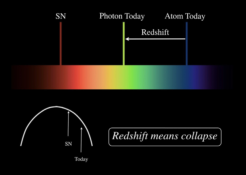
Edwin Hubble observed that the color of light emitted by atoms from distant galaxies is redder than similar atoms emit today on earth. The farther away the galaxy, the greater this redshift. This redshift has been interpreted as a result of an expanding universe “stretching” the photons as described by Alexander Friedmann’s solution to Einstein’s general theory of relativity. But this interpretation of color shift of photons ignores the fact that atoms as well as photons change with the universe. Atomic emissions change twice as much as photon wavelengths do. When atomic emission changes are included, Hubble redshift implies that the Friedmann universe is collapsing, not expanding. This conclusion is confirmed by modern observations.
Introduction
In Maxwell’s equations vacuum permittivity, ε, is the scalar that determines the speed of light and the strength of electrical fields. Einstein’s discovery that ε changes with gravity means that both the wavelengths of photons and the wavelengths of photons emitted by atoms change with spacetime curvature in general relativity. In Friedmann spacetime, vacuum permittivity, ε, is directly proportional to the Friedmann radius so ε changes with time. As the size of the Friedmann universe evolves, the changing strength of the electrical force between charges shifts atomic energy levels, changing the wavelengths of emitted light. The wavelengths of photons also change but only half as much. This difference in evolution of atomic emissions and photons reverses the interpretation of Hubble redshift Sumner [1]. Our Friedmann universe is closed and collapsing (Figure 1).
Mathematical Models
Einstein’s Solution
In his study of Maxwell’s equations in an uniformly accelerated coordinate system, Einstein [2] concluded that the velocity of light in special relativity, c, is reduced to c∗, the local coordinate velocity of light in the accelerated system. Einstein [3] found in an accelerated system which corresponds locally to the gravitational field of a point mass $$ ^ {*} = c \left(1 + \frac {\Phi}{c ^ {2}}\right), $$ (1)
2 * 1 , c c c where Φ is the Newtonian gravitational potential $$ \Phi = - \frac {k m}{r} (2) $$ m is the mass of the object creating the gravitational field at a distance r. k is the gravitational constant. The connection between Einstein’s result, equation (1), and the strength of the electrical field comes from the definition of relative vacuum permittivity ε, $$ \varepsilon = \frac {c}{c ^ {*}} [ 3 ] $$ Combining equations (1), (2), and (3) gives Einstein’s value for ε, ( )
1 $$ \varepsilon (r) = \frac {1}{\left(1 - \frac {k m}{r c ^ {2}}\right)} $$
(4)
1 r km rc
2 Møller [4] and Landau & Lifshitz [5] studied the effects of curved spacetime on Maxwell’s equations. Both proved that in a static gravitational field the electromagnetic field equations take the form of Maxwell’s phenomenological equations in a medium at rest with ( ) 1 $$ \varepsilon (r) = \frac {1}{\sqrt {g 0 0}} (5) $$ g_00 is the time component of the metric tensor _gµν.
Einstein’s pre-general relativity result, equation (4), is the first approximation to the exact relativistic equation (5), ( )
1 1 1 ε = = ≈ − −
(6) r km g km rc rc
00 2 1 1
2 2
Friedmann Solution
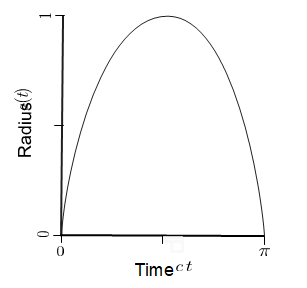
Friedmann [6] published a closed universe solution to Einstein’s theory of general relativity without a cosmological constant. The Friedmann universe rapidly expands from a singularity, slowing until it reaches a maximum size before accelerating back to a singularity (Figure 2).
$$ d s ^ {2} = c ^ {2} d t ^ {2} - a ^ {2} (t) \left[ \frac {d r ^ {2}}{\left(1 - r ^ {2}\right)} + r ^ {2} \left(d \theta^ {2} + \sin^ {2} \theta d \varphi^ {2}\right) \right], $$ ( ) ( ) ( )
2 2 2 2 2 2 2 2 2
2 sin 1 , (7) and homogeneous, incoherent matter, conserved in amount and exerting negligible pressure. His solution is the cycloid shown in Figure 2, $$ a = \frac {\alpha}{2} \left(1 - \cos \psi\right) \quad c t = \frac {\alpha}{2} \left(\psi - \sin \psi\right) \tag {8} $$ where α is a constant and 0 ≤ ψ ≤ 2π [7].
Sumner [1] examined Maxwell’s equations in Friedmann geometry and found that ε changes in time along with spacetime curvature, ε(t) = a(t). (9) a(t) is the radius of the Friedmann universe defined above with α = 1.
Local Mathematical Coordinates
The effects of spacetime curvature in nature are often explained as gravitational forces or simply ignored. The extraordinary success of the special theory of relativity confirms this approach. But spacetime is never precisely flat as ubiquitous gravity clearly shows. Flat spacetime exists only in mathematical models. Every spacetime in nature is curved.
To understand the effects of spacetime curvature on atoms and photons, a coordinate system that includes spacetime curvature is necessary. The method used by Einstein, Meller, Landau, Lifshitz, and Sumner is adopted where a local pseudo-Cartesian coordinate system is used with the vacuum permittivity $\varepsilon(x^0)$ determined by the general relativistic geometry at that spacetime point. Specifically,
$$ds^2 = \frac{c^2}{\varepsilon^2(x^0)} dt^2 - \left[ dr^2 + r^2 \left( d\theta^2 + \sin^2 \theta D\phi^2 \right) \right]$$
If the variation in $\varepsilon(x^0)$ in the region of interest is ignored, equation (10) is just the metric of special relativity with a velocity of light $c/\varepsilon(x^0)$. If $\varepsilon(x^0) = 1$ the result is special relativity with spacetime curvature ignored.
**Changes in Atoms and Photons**
The Bohr radius $a_0$ of a hydrogen atom in its ground state
$$t = \frac{2a_0}{m} \left( \frac{x}{m} \right)^{1/2}$$
$\varepsilon_0 = 8.854187817 \times 10^{-11} \text{ F/m}$ (farads per meter) [8] is the defined value of $\varepsilon_0$. $m$ is the mass of the electron, $e$ is the charge of the electron, and $h$ is Planck’s constant $h$ divided by $2\pi$. These are assumed to remain constant as spacetime curvature changes.
The change in Bohr radius $a_0$ as $t$ changes is
$$\frac{a_0(t_1)}{a_0(t_2)} = \frac{\varepsilon(t_1)}{\varepsilon(t_2)}$$
The characteristic wavelength $\lambda_e$ emitted by a hydrogen atom during the transition between the quantum numbers $n_1$ and $n_2$ is
$$\lambda_e(t) = \frac{8\varepsilon_0^2 \varepsilon^2(t) \hbar^2 c}{me^4} \left( \frac{n_1^2 n_2^2}{n_2^2 - n_1^2} \right)$$
$c$ in equation (13) comes from the defining relationship between $\lambda$ and $v$, $\lambda v = c$.
The change in $\lambda_e(t)$ as $t$ changes is
$$\frac{\lambda_e(t_1)}{\lambda_e(t_2)} = \frac{\varepsilon^2(t_1)}{\varepsilon^2(t_2)}$$
Consider the Compton wavelength, $\lambda_e$ of a particle with mass $m_p$
$$\lambda_c(t) = \frac{h}{m_p c^*} \left( \frac{h \varepsilon(t)}{m_p c} \right)$$
The change in $\lambda_e(t)$ as $t$ changes is
$$\frac{\lambda_c(t_1)}{\lambda_c(t_2)} = \frac{\varepsilon(t_1)}{\varepsilon(t_2)}$$
The Compton wavelength of a particle is equivalent to the wavelength of a photon of the same energy as the particle. Compton and photon wavelengths have the same $\varepsilon(t)$ dependency that the Bohr radius has. The wavelength change for a photon is
$$\frac{\lambda_c(t_1)}{\lambda_c(t_2)} = \frac{\varepsilon(t_1)}{\varepsilon(t_2)}$$
**Gravitational Redshift**
The following notation is used. The wavelength of a photon $\lambda$ emitted at $t_1$ and examined at $t_1$ will be written $\lambda(t_1, t_2)$. The wavelength of a photon $\lambda$ emitted at $t_1$ and examined at $t_2$ will be written $\lambda(t_1, t_2)$.
The traditional redshift $z$ formula assumes that atomic emissions do not evolve, $\lambda(t_2, t_2) = \lambda(t_1, t_1)$, but that photons do (Equation (17)).
$$z = \frac{\lambda(t_1, t_2) - \lambda(t_1, t_1)}{\lambda(t_1, t_1)} = \frac{\varepsilon(t_2)}{\varepsilon(t_1)} - 1$$
$t_2$ is the observer’s location and $t_1$ is the location at the time of emission.
Since atomic emissions do evolve with spacetime geometry, a new redshift variable $\zeta$ (the Greek letter zeta) is defined to match what is done experimentally.
$$\zeta = \frac{\lambda(t_1 - t_2) - \lambda(t_2 - t_2)}{\lambda(t_2 - t_2)}$$
$t_2$ is the observer’s location and $t_1$ is the location at the time of emission.
$$\zeta = \frac{\varepsilon(t_1)}{\varepsilon(t_2)} - 1$$
Substituting ε(t) = a(t) into equation (20) gives the redshift ζ for Friedmann geometry, ( ) ( )
1 1 a t $$ \varsigma = \frac {a \left(t _ {1}\right)}{a \left(t _ {1}\right)} - 1 \tag {21} $$
1 Hubble redshift (ζ > 0) implies a(t_1) > a_(t_2). The universe was larger in the past, _a(t_1), than it is now, _a(_t_2). This puts us somewhere on the collapsing half of the curve in Figure 2. The logic is simple. Since Hubble shifts are red (ζ > 0), the Friedmann universe is collapsing. If Hubble shifts were blue (ζ < 0), the Friedmann universe would be expanding.
Analyzing Hubble Redshifts
The analysis of redshift observations must include the changes in atomic emissions in addition to the changes in photons. Astronomers measure the redshift defined by ζ, equation (21). The following derivation is similar to the one made when atomic evolution is ignored and the universe is assumed to be expanding [9], but is different because ζ not z describes the observed redshift and some choices in signs are made differently when the universe is contracting [10]. It is assumed that observed photons were emitted after contraction began.
The mathematical coordinate distance r to a source can be shown to be a function of the observed redshift ζ of the source and the deceleration parameter qo in the following way.
Setting ds = 0 in the Friedmann metric, equation (7), gives ( )
− = a t dr cdt (22)
1 2 2 1 ( )
− r The source is located at the spatial coordinates (r_1,0,0) with emission at time _t_1 and the observer is at (0,0,_0) with reception at time _t_2.
t dt dr c r a t r t r $$ c \int_ {t _ {1}} ^ {t _ {2}} \frac {d t}{a (t)} = \int_ {0} ^ {r _ {1}} \frac {d r}{\left(1 - r ^ {2}\right) ^ {1 / 2}} = \sin^ {- 1} r _ {1} \tag {23} $$
1 1 1 0 2 2 sin 1
2 1 ( ) ( )
1 Substituting a(t) and dt calculated from the Friedmann solution, equation (8), gives $$ r _ {1} = \sin \left(\psi_ {2} - \psi_ {1}\right). \tag {24} $$ The Friedmann equation for the closed universe is [9]
2 2 1 a c a α = −
(25) The Hubble constant H and the deceleration parameter q are defined by ( ) ( ) ( ) ( ) 2 ( ) ( ) , ( ) $$ H (t) = \frac {\dot {a} (t)}{a (t)}, \frac {\ddot {a} (t)}{a (t)} = - q (t) H ^ {2} (t). \tag {26} $$ “ ˙ ” indicates time derivative. H is negative and q is greater than 1_/2 for a closed, collapsing universe. Present day values are denoted by _Ho and qo.
α, the constant in equations (8), may be written [9]
2 q c (27)
| 3 (2q −1) 2 | H 0 |
|---|
Solving for ψ2 and ψ1 in terms of ζ and qo and substituting into equation (24) gives ( ) ( )( )
1 2 0 0 $$ \begin{array}{l} = \frac {\left(2 q _ {0} - 1\right) ^ {1 / 2}}{q _ {0}} \left[ \varsigma - \frac {\left(1 + \varsigma\right) \left(1 - q _ {0}\right)}{q _ {0}} \right] _ {1 / 2} + \\ \frac {1 - q _ {0}}{q _ {0}} \left\{1 - \left[ \varsigma - \frac {\left(1 + \varsigma\right) \left(1 - q _ {0}\right)}{q _ {0}} \right] ^ {2} \right\} ^ {1 / 2} \\ \end{array} $$ ς ς
2 1 1 1 q q r q q
0 0 The flux f of photons is related to the luminosity L of the source and to its luminosity distance DL by the equation $$ f = \frac {L}{4 \pi D _ {L} ^ {2}} \tag {29} $$
2 4 L
DL is determined in the following way. Calculate the observed flux f by noting that L, the actual luminosity of the source, is changed by a factor of a(t_2)/a_(t_1) because of the apparent change of the photon’s energy and changed by another factor of _a(t_2)/a_(t_1) because of the changes in time in the local metric, equation (10). The distance to the source is _r_1 _a(_t_2). This gives an observed flux of ( ) ( )
2 2 $$ f = \frac {L \frac {a ^ {2} \left(t _ {2}\right)}{a ^ {2} \left(t _ {1}\right)}}{4 \pi r _ {1} ^ {2} a ^ {2} \left(t _ {2}\right)} \tag {30} $$
2 1 ( )
2 2 1 2 4 Combining equations (29) and (30) using (21) gives $$ D _ {L} = r _ {1} a \left(t _ {2}\right) \left(1 + \zeta\right). \tag {31} $$ a(_t_2) is [9]
− = − ( )
1 c a t H q (32)
( )
2 1 2 0 0
2 1
Substituting equations (28) and (32) into (31) gives ( )( )
$$ = \frac {- c}{H _ {0}} \frac {\left(1 + \varsigma\right)}{q _ {0}} \left\{ \begin{array}{l} \left[ \varsigma - \frac {\left(1 + \varsigma\right) \left(1 - q _ {0}\right)}{q _ {0}} \right] + \\ \frac {\left(1 - q _ {0}\right)}{\left(2 q _ {0} - 1\right) ^ {1 / 2}} \left(1 - \left[ \varsigma - \frac {\left(1 + \varsigma\right) \left(1 - q _ {0}\right)}{q _ {0}} \right] ^ {2} \right] ^ {1 / 2} \end{array} \right\} $$ ς ς ς ς ς
1 1 q
0 ( ) q c D q q H q q q
( ) (33) The relationship between distance modulus (the difference between the apparent magnitude m and absolute magnitude M of a celestial object) and luminosity distance, DL, is m − M = 5log10 (34) The Hubble constant Ho (negative for the contracting half of the curve) and the deceleration parameter qo (which must be > 1_/2 characterizing a closed Friedmann universe) are then varied to find best least-squared fits to Hubble redshift observations of ζ and _m − M using equations (33) and (34).
Fit to Pantheon Sn Redshift Data
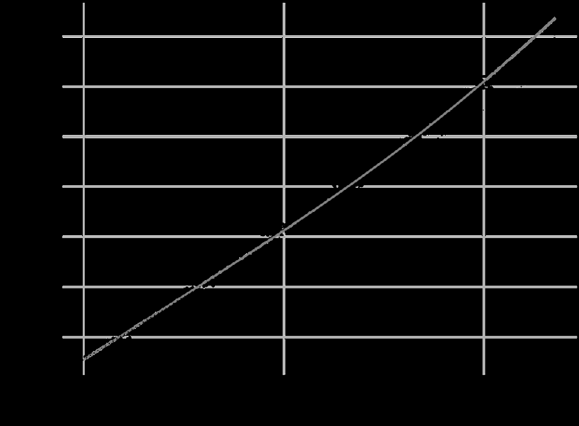
The Pantheon redshift data of 1048 supernovas [11] were analyzed assuming that both atoms and photons change. The Hubble constant and deceleration parameter were the only variables, see Figure 3.
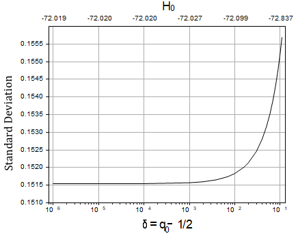
Figure 3: The solid line is the fit to the Pantheon redshift data with the parameters Ho = -72.10±0.75 km s−1 Mpc−1 and 1_/2 < q_o < 0_.51. The dotted straight line is included to visually clarify the upward curve (or “acceleration”) of the data and fit. The average data error is 0.1418. The standard deviation for this fit is 0._1515.
Since this Friedmann universe is closed, qo > 1_/2. Every search conducted found a lower standard deviation when _qo was closer to 1_/2. No lower limit for δ = (_qo − 1_/2) was found and the upper limit 0.51 was chosen because there is little change in the quality of fit with smaller _qo, hence 1_/2 < q_o < 0_._51. This is illustrated in Figure 4.
Our Universe
0 2 3 H −estimates the time until collapse, tc, of the Friedmann
1 universe when qo is this close to ½. For Ho = −72.10_kms_−1_Mpc_−1, tc = 9.05 billion years.
The age of the universe, tA, can be estimated from the magnitude-redshift data [9] (with two signs changed to reflect contraction), $$ 1 = \frac {- 1}{H _ {0}} \left[ \frac {1}{2 q _ {0} - 1} + \frac {q _ {0}}{\left(2 q _ {0} - 1\right) ^ {3 / 2}} \cos^ {- 1} \frac {1 - q _ {0}}{q _ {0}} \right] $$
1 1 1 cos 2 1 2 1
A q q t H q q q
1 0 0 3 2 0 0 0 0
(35) ( ) A value for cos−1 corresponding to the fourth quadrant must be used. For Ho = −72_.10_kms−1_Mpc_−1 and qo = 0_.51, _tA = 1_._54 × 104 billion years.
For qo = 1_/2, equation 35 gives an age of _tA = ∞ as it should for a flat universe. While the Pantheon data makes a persuasive case that our universe is closed, nearly flat, and very old, it does not give definitive answers to the questions “How flat is the universe?” and “How old is the universe?”
Velocity of Light
Einstein [2] concluded that the velocity of light in special relativity, c, is reduced in an uniformly accelerated coordinate system to c∗, the local coordinate velocity of light. The ratio c/ c∗ is relative vacuum permittivity ε, equation 3.
For Friedmann geometry ε(t) = a(t). Equation 3 gives c∗(t)a(t) = c∗(to)a(to), (36) where a(to) is the radius of the universe when the velocity of light is c∗(to) = c = 2_._998 × 1010 cm/sec.
At the Big Bang (when a(t) = 0), the local coordinate velocity c∗(t) was infinite before dropping to its current value c at 9.05 × 10⁹ years, before reaching a minimum at full expansion, and then increasing back toward infinity again at collapse.
The symmetry of the Friedmann cycloid is used to equate the velocity and radius during the expansion period to the current collapsing data for Ho, qo, and to = tc derived from Ho. Equations 8 then give ψo, a(to) and α.
Mathematics and Physics
The mathematics of general relativity isn’t a physical theory until mathematical concepts such as gµν and xµ are linked by axioms to specific physical measurements. Albert Einstein took this step, just as he did for special relativity, by asserting that measurements made with rigid meter sticks and balance clocks are equivalent to the mathematical distances and times of general relativity. Assuming a rigid meter stick is equivalent to assuming that atoms never change. Even as he did this Einstein had qualms about his choices. From Einstein’s 1921 Nobel Lecture [12]: ... it would be logically more correct to begin with the whole of the laws and ... to put the unambiguous relation to the world of experience last instead of already fulfilling it in an imperfect form for an artificially isolated part, namely the space-time metric. We are not, however, sufficiently advanced in our knowledge of Nature’s elementary laws to adopt this more perfect method without going out of our depth [12].
It is intriguing that it was Einstein who discovered vacuum permittivity depends on gravity. In 1907, there was no general relativity, no Bohr atom, and no clear understanding of photons. When these theories were later in place, the connection provided by vacuum permittivity between spacetime curvature and atomic structure was overlooked. Einstein [13] knew that the “tools for measurement do not lead an independent existence alongside of the objects implicated by the field equations.” What he did not realize was that the solution was already in his 1907 paper and that there was no need of “going out of our depth” to create the more complete general relativity he wanted, where the “tools for measurement” depend on spacetime exactly as “other objects implicated by the field-equations.” Schrodinger [14] published his seminal discovery that every quantum wavelength expands and contracts in proportion to the radius of a closed Friedmann universe. Schrodinger argued that if spacetime is curved as general relativity requires, then its effects on quantum processes must not be dismissed without careful investigation. Using the equations of relativistic quantum mechanics, Schrodinger found that the plane-wave eigenfunctions characteristic of flat spacetimes are replaced in the curved spacetime of the closed Friedmann universe by wave functions with wavelengths that are directly proportional to the Friedmann radius.
This means that every eigenfunction changes wavelength as the radius of the universe changes. The quantum systems they describe change as well. In an expanding universe quantum systems expand. In a contracting universe they contract. The assumption is often made that small quantum systems are isolated and that their properties remain constant as the Friedmann universe evolves. This assumption is incompatible with relativistic quantum mechanics and with the curved spacetime of general relativity as Schrodinger proved [15].
Schrodinger had a deep understanding of both wave mechanics and general relativity. Like most physicists, Schrodinger “knew” Hubble redshift meant that the universe is expanding, a hangover from the pre-relativistic interpretations of redshifts originally made by Slipher [16] and Hubble [17] who tentatively assumed that all galactic redshifts are solely Doppler shifted photons. It is interesting to speculate how long it would have taken Schrodinger to correctly interpret Hubble redshift if he had asked himself the question: “Would the changes in atoms and photons that I found change my interpretation of Hubble redshift?” Feynman [18] was correct when he observed that “Physics is not mathematics, and mathematics is not physics ... mathematicians prepare abstract reasoning that’s ready to be used if you will only have a set of axioms about the real world ...” Assuming that meter sticks are made of atoms that never change does not belong in that set, nor does assuming that the speed of light is a constant [19, 20, 21, 22].
Conclusion
Vacuum permittivity, a measure of the strength of electric fields and light velocity in a vacuum, changes with the spacetime curvature of general relativity. This changes atomic energy levels, photon wavelengths, and the velocity of light. For Friedmann geometry a comparison of photons emitted long ago to those emitted today predicts that Hubble redshifts result from a universe accelerating in collapse.
This is confirmed by the Pantheon redshift data where no modifications to general relativity or to Friedmann’s [6] assumptions are necessary to explain Hubble redshift. Assuming changes in both atomic emissions and photon wavelengths and varying only Ho and qo gives Ho = -72.10±0.75 km s−1 Mpc−1 and 1_/2 < q_o < 0_.51. The average data error is 0.1418. For these fit parameters the standard deviation is 0.1515. The changes in atoms and photons derived here agree with Schrodinger’s 1939 conclusion that quantum wave functions expand and contract with the radius of a closed Friedmann universe. The velocity of light is inversely proportional to vacuum permittivity which is proportional to the radius of the Friedmann universe. Light velocity was infinite at the Big Bang, dropped to its current value _c a_t 9.05 × 10⁹ years on its way to a minimum at full expansion. _c will be infinite again in 9.05 × 10⁹ years. The estimated age of the universe is tA = 1_._54 × 104 billion years.
Acknowledgments
The author is grateful to Sumner DY and Vityaev EE for invaluable collaborations and to Feigl EO and Hornbein TF for helpful comments and suggestions. Special thanks go to the curators of the superb Pantheon SN data set and to Riess AG who recommended it. The Python program curve fit from scipy.optimize was used with equations (33) and (34) to analyze the Pantheon data, Scolnic [11]. https://dx.doi.org/10.17909/T95Q4X
References
-
Sumner W (1994) On the variation of vacuum permittivity in Friedmann universes. ApJ 429(2): 491-498.
-
Einstein A (1907) über das Relativitätsprinzip und die aus demselben gezogenen Folgerungen. Jahrbuch der Radioaktivit¨at und Elektronik 4: 411-462.
-
Einstein A (1989) The Collected Papers of Albert Einstein. Volume 2, Princeton University Press, Princeton.
-
Møller C (1952) The Theory of Relativity. Clarendon Press, Oxford.
-
Landau L, Lifshitz E (1975) The Classical Theory of Fields. Volume 2, Pergamon Press, Oxford.
-
Friedmann A (1922) About the curvature of space. Z Phys 10: 377-386.
-
Tolman RC (1934) Relativity, Thermodynamics, and Cosmology. Clarendon Press, Oxford.
-
Leighto RB (1959) Principles of Modern Physics. McGraw-Hill, New York.
-
Narlikar J (1983) An Introduction to Cosmology. 3rd(Edn.), Cambridge University Press, Cambridge.
-
Sumner WQ, Vityaev EE (2000) Hubble Redshift. Astrophysics, pp: 8.
-
Scolnic DM, Jones DO, Rest A, Pan YC, Chornock R, et al. (2018) The Complete Light-curve Sample of Spectroscopically Confirmed SNe Ia from Pan-STARRS1 and Cosmological Constraints from the Combined Pantheon Sample. ApJ 859(2): 1-28.
-
Einstein A (1967) Nobel Lectures, Physics 1901-1921. Elsevier Publishing Company, Amsterdam, pp: 482-490.
-
Schilpp PA, Einstein A (1949) Albert Einstein: Philosopher-Scientist. 1st(Edn.), Evanston Ill.
-
Schrodinger E (1939) The proper vibrations of the expanding universe. Physica 6(7-12): 899-912.
-
Sumner WQ, Sumner DY (2000) Coevolution of Quantum Wave Functions and the Friedmann Universe. arXiv:0704.2791v1, pp: 8.
-
Slipher V (1917) Nebulae. Proc Amer Phil Soc 56: 403- 409.
-
Hubble E (1929) A relation between distance and radial velocity among extra-galactic nebulae. Proceedings of the National Academy of Science 15(3): 168-173.
-
Feynman R (1967) The Character of Physical Law. The M.I.T. Press, Cambridge.
-
Einstein A (1911) On the influence of gravity on the propagation of light. Annalen der Physik 340(10): 898- 908.
-
Einstein A (1993) The Collected Papers of Albert Einstein. Volume 3, Princeton University Press, Princeton.
-
Pauli W (1958) Theory of Relativity. Pergamon Press, Oxford.
-
Schrodinger E (1956) Expanding Universes. Cambridge University Press, Cambridge.
- Sense, Gravity, Parity & Chirality in Mathematical Physics
- Quantum Lattice Simulations PHYSICS: Microcircuit Particle Formation and Observable Macroscopic Irreversible Time - A Discrete Lagrangian with Cellular Automata Framework
- Quantum Biology from Biomacromolecule to Cell, and Central Dogma Described by Quantum Theory
- Focus, Agility, Speed and Technology (FAST) for Sustainability and Growth
- Square Root Metric Geometry and Pati-Salam Model in Curved Space-Time
- A Simple System Demonstrating the Mpemba Effect in Classical Mechanics