Relativistic Solutions of Dirac Equation with the Molecular Hua Potential in the Spin Symmetry Limit
The study presents solutions of Dirac equation with the Molecular Hua potential energy model using the Formula method. In the non-relativistic limit, the relativistic energy equation becomes the non-relativistic rotation-vibrational energy expression. Numerical results for some molecules are also presented. Interestingly, our results agree with those in literature.
Introduction
The solutions of wave equations are known to be vital in quantum mechanics and related areas of physics. The reason is because the solutions have all the relevant parameters required to evaluate the associated properties of a physical system under consideration. Reports on the nonrelativistic rotational vibrational energies of molecules obtained from solutions of Schrodinger equation in various potential models have been presented [1, 2, 3, 4, 5]. It has been established that relativistic interactions are essential for an accurate determination of the rotation-vibration energy spectra of molecules by using quantum mechanical techniques [6]. Recently, by solving Dirac equation with General molecular potential, Improved Tietz potential and Improved Rosen-Morse potential, some authors investigated the relativistic rotation-vibrational energies for $5^1\Delta_g$ state of Na$_2$ molecule, the $X^2 \sum^+$ state of the CP molecule and $3^3 \sum^-$ state of the Cs$_2$ molecule, and observed that nonrelativistic energies decreases as a result of relativistic effects [7, 8, 9].
In this paper, we attempt to investigate the solutions of Dirac equation with the Hua potential energy model. We also explore the relativistic effects of rotational vibrational energies for some molecules.
Recently, Hassanabadi H, et al. [10] studied the Schrodinger equation with Hua potential using the super symmetry quantum mechanics. Also, a similar form of Hua potential has been reported by Hua W, et al. [11], to study the rotation-vibration spectrum of different molecules. The Hua potential can be used in describing the energy levels of diatomic molecules, hence motivation for this work. The Hua potential is expressed as [12, 13].
$$U_H = V_0 \left( \frac{1 - e^{-b_h(t-r_h)}}{1 - qe^{-b_h(t-r_h)}} \right)^2, \quad b_h = \beta (1 - c_h),$$ where V0 , re, q and β are respectively the potential depth, bond length, deformation parameter and Morse constant. The work is drafted as: The Formula method is presented in Section 5, Section 6 is a review of Dirac equation under spin symmetry [14]. The bound state solutions are given in Section 7. Discussion comes in Section 9. Finally, conclusion is presented in Section 10.
Formula Method
The Formula method is applied by considering the equation.
α α ψ ψ α ξ ξ ξ ψ α $$ \begin{array}{l} \frac {d ^ {2} \psi (s)}{d s ^ {2}} + \frac {\alpha_ {1} - \alpha_ {2} s}{s \left(1 - \alpha_ {3} s\right)} \frac {d \psi (s)}{d s} \\ + \frac {\xi_ {1} s ^ {2} + \xi_ {2} s + \xi_ {3}}{s ^ {2} \left(1 - \alpha_ {3} s\right) ^ {2}} \psi (s) = 0. \tag {2} \\ \end{array} $$
The energy and the wave function are derived respectively,
from the equations
2 1 2 2 2 3 1 2 3 2 2 3
s d s d s s s ds dss s s s s ( ) ( ) (1 )
( ) 0. (1 )
2 2 2 2 2 4 5 2 3 2 1 2 3 2 5 3 2
$$ \left[ \frac {\alpha_ {4} ^ {2} - \alpha_ {5} ^ {2} - \left[ \frac {1 - 2 n}{2} - \frac {1}{2 \alpha_ {3} ^ {2}} \left(\alpha_ {2} - \sqrt {\left(\alpha_ {3} - \alpha_ {2}\right) ^ {2} - 4 \xi_ {1}}\right) \right] ^ {2}}{2 \left[ \frac {1 - 2 n}{2} - \frac {1}{2 \alpha_ {3} ^ {2}} \left(\alpha_ {2} - \sqrt {\left(\alpha_ {3} - \alpha_ {2}\right) ^ {2} - 4 \xi_ {1}}\right) \right]} ^ {2} - \alpha_ {5} ^ {2} = 0, \alpha_ {3} \neq 0 \tag {3} $$ ( )
1 2 1 4 2 2 0, 0 1 2 1 2 4 2 2
n α α α α α ξ α α α ( )
n α α α ξ α
$$ F _ {1} \left(- n, n + 2 \left(\alpha_ {4} + \alpha_ {5}\right) + \frac {\alpha_ {2}}{\alpha_ {3}} - 1; 2 \alpha_ {4} + \alpha_ {1}; \alpha_ {3} s\right), \tag {4} $$ α α α α α α α ( )
2 4 1 1 $$ = \frac {\left(1 - \alpha_ {1}\right) + \sqrt {\left(1 - \alpha_ {1}\right) ^ {2} - 4}}{2} $$ ξ α α α
2 $$ = \frac {1}{2} + \frac {\alpha_ {1}}{2} - \frac {\alpha_ {2}}{2 \alpha} + \sqrt {\left(\frac {1}{2} + \frac {\alpha_ {1}}{2} - \right.} $$ $$ \left. \frac {1}{4}\right) ^ {2} - \left(\frac {\xi_ {1}}{\alpha_ {3} ^ {2}} + \frac {\xi_ {2}}{\alpha_ {3}} + \varphi\right) $$
2 2 2 1 2 2 2 1
ξ α ξ α ξ α α α α α α α
$$ \alpha_ {1} = 1, \alpha_ {2} = \alpha_ {3} = q, $$
, we put forward a
simplified energy equation from Equation (3) ( ) ( )
2 2 2 2 ξ ξ ξ ξ ξ ξ $$ \sqrt {- \xi_ {3}} \left(q + \sqrt {q ^ {2} - 4 \left(\xi_ {1} + q \xi_ {2} + q ^ {2} \xi_ {3}\right)} + 2 q n\right) = q ^ {2} \xi_ {3} - \xi_ {1} - q ^ {2} n (n + 1 $$
4 2 1 3 1 2 3 3 1 2 1 4 4 1 2 3 1 2 3 2 2
q q q q q qn q q n n ( ) ( )
q qn q q q q q q
2 2 2 2 ξ ξ ξ ξ ξ ξ $$ - q n \sqrt {q ^ {2} - 4 \left(\xi_ {1} + q \xi_ {2} + q ^ {2} \xi_ {3}\right)} - \left(\frac {q}{2} + \frac {1}{2} \sqrt {q ^ {2} - 4 \left(\xi_ {1} + q \xi_ {2} + q ^ {2}\right)}\right) $$ (6)
Dirac Equation
The Dirac equation with scalar, S(r) and vector potential, V(r) is given as $$ \begin{array}{l} \hat {H} _ {D} \Psi (r) = E _ {v k} \Psi (r) \\ \hat {H} _ {D} = c \alpha . \overrightarrow {p} + \beta \left(\mu c ^ {2} + S (r)\right) + V \\ \end{array} $$
2 ( ) ( ) H r E r D vk H c p c S r V r α β µ . ( ( )) ( )
D
, (7) $$ \mathrm {w h e r e} \mu , E _ {v k}, \overrightarrow {p} = - i \hbar \overrightarrow {\nabla} $$
are the reduced mass, relativistic energy, and momentum operator respectively. β α, are the
4×4 Dirac matrices given by
$$ = \left( \begin{array}{c c} 0 & \sigma_ {i} \\ \sigma_ {i} & 0 \end{array} \right) $$ i σ σ α
0 β I
$$ \gamma = \left( \begin{array}{c c} I & 0 \\ 0 & - I \end{array} \right) $$
0 i , , (8) Where I is the 2×2 matrix and i σ is the Pauli matrices given as
1 0 $$ = \left( \begin{array}{c c} 0 & - i \\ i & 0 \end{array} \right) $$
$$ = \left( \begin{array}{c c} 1 & 0 \\ 0 & - 1 \end{array} \right) $$
2 i i σ
$$ = \left( \begin{array}{c c} 0 & 1 \\ 1 & 0 \end{array} \right) $$
1 σ
3 σ , , (9) The spinor, ) (r Ψ can be written as
l n jm l n jm θ φ ( ) ( , ) 1 ( ) ( ) ( , )
F r Y
κ $$ \Psi (r) = \frac {1}{r} \left| i G _ {n \kappa} (r) Y _ {i m} ^ {\tilde {l}} \right. $$ θ φ r iG r Y r κ , (10) with ) (r Fnκ and ) (r Gnκ as the upper and lower components of the Dirac spinors. ( , ) jml Y θ φ is the spherical harmonic of the spin component and ( , ) jml Y θ φ is the spherical harmonic of the pseudo spin component. l and l~ are the orbital and pseudo-orbital quantum numbers, while κ and m are the spin-orbit coupling operator and projection on z-axis. If the spinor in Equation (10) is used, we deduce the following coupled radial differential equations from the Dirac equation − +
2 µ $$ 0 = \frac {\left(\mu c ^ {2} - E _ {v k} + \Sigma\right)}{h c} $$
( ) ( ) ( )
c r E G r F r c c r E F r G r c vk d n n dr r κ κ κ η
2 + −∆ = µ ( ) ( ) ( )
vk d n n dr r κ κ κ η
(11)
If ) (r Fnκ is eliminated in favor of ) (r Gnκ , we derive two uncoupled differential equations of the form
2 2 2 µ µ κ κ νκ νκ − + Σ + −∆ + − −
( ( ))( ( )) ( ) ( 1) ( ) ( )
r r d F r c c E E F r F r dr r c κ κ κ n n n
2 2 2 2 η ∆ + + = + −∆
κ ( ) ( ) d r d F r dr dr r κ n
0, ( ( )) µ νκ
2 r c E (12)
2 2 2 µ µ κ κ νκ νκ − + Σ + −∆ − − −
( ( ))( ( )) ( ) ( 1) ( ) ( )
r r d G r c c E E G r G r dr r c κ κ κ n n n
2 2 2 2 η Σ − − = − + Σ
κ ( ) ( ) d r d G r dr dr r κ n
0, ( ( )) µ νκ
2 r c E (13)
κ κ κ κ + = + − = + ∆
( 1) ( 1), ( 1) ( 1), ( )
l l l l r .
where = − Σ = +
( ) ( ), ( ) ( ) ( )
V r S r r V r S r
Bound State Solutions
∆ = ∆ = constant. In the non- In spin symmetry, ( ) 0; ( ) d r r C dr relativistic limit, Equation (12) reduces to a Schrodinger form with 2_V(r) in light of the exact symmetry _V(r) = S(r). Adopting a proposal by Alhaidari AD, et al. [15], and setting S(r) = UH, V(r) = Cs + UH(r), expansion of Equation (12) gives + − + + − + −
2 2 κ κ µ κ κ νκ ( ) ( ) ( 1) ( ) 2
n n H d F r c C C E s s F r U dr c r
2 2 2 2 η ( )
− + − = −
2
2 4 2 µ µ νκ νκ κ C c c E E s F r n c ( ).
2 2 η (14) To solve Equation (14), we adopt an approximation − − − − ( ) 2 ( ) b r r b r r e e h h
1 1 e e D D D r r e qe qe ≈ + + − −
− − − −
0 1 2 2 2 ( ) ( )
b r re h b r r h e
1 1 (15) The approximation is only valid for 1 b re h qe ≥ . We can set er er r x er h b − = = , α in Equation (14) and expand up to x_2 term, we have ) 3 ( ) 1( 3 1 1 _q q q D + − − − + =
0 α α ) 1( 3 ) 2 ( ) 1( 2
− − + − =
2 1 q q q D
α α
3 ) 1( ) 1( 3 ) 1(
q q q D + − − − =
2 α α (16) Substituting Equation (15) in Equation (14) and rearranging gives − − − − − − − − − − − − ( )
2 b r r h e C s − − + +
1 2 1 ( ) e V
ε ε ( )
1 0 2 b r r h e
− qe d F r n dr e e D D D r qe qe
2 κ ( ) ( )
= + ( ) 0, F r nκ
2 2 b r r b r r h e h e + − + +
κ κ ( 1) 2 1 1
( )
0 1 2 2 b r r e b r r h e h e − −
(17) where
2 µ ε + − =
( ) c E C s νκ
2 2
1 c η
2 2 4 2 µ µ ε − + − =
E c c E C s νκ νκ
2 2 2 c η (18) To solve Equation (17), we use the transformation ) ( er r h b e s − − = , which gives
2
2 ( ) (1 ) ( ) 0 (1 ) (1 ) ds dF Ps n n n ds d F s qs s Qs R F s qs s qs κ κ κ − + + + + = − − , (19) where,
+ − − − + − + + − =
)1 ( 2 )1 ( )1 ( 1
r D q V C q r D r D q q b P
κ κ ε ε κ κ κ κ ε
2 2 2 1 2 2
s e e h
e + − + + − + =
)1 ( )1 ( 2 2 2 1
r D r D q q V C q b Q
κ κ κ κ ε ε ε
.
2 1 2 0 2 0 1 1
e e s h
+ − − − − =
)1 ( 2 1 r D V C b R
κ κ ε ε ε
2 0 0 1 1 2
s h e (20) The constants are calculated from Equation (5) as
, , ,1 R q − = = = =
α α α α
4 3 2 1
| 1 2q | 4 κ(κ+1)D εV (q−1)2 + 2 +q2 b 2 1 0 r2 h e |
|---|
Using Eqs. (6) and (4), the relativistic energy and unnormalized eigen function are derived as + − + + − + − + − + = + + + − + + − + + + + − + + −
2 2 4 2 2 µ µ µ κ κ E c c E C c E s C s D C s V r c c V c E D q s q qn n b r c c E C s n c e ( ) ( 1) 0 2 2 ( ) ( 1) 1 ( 1) ( 1) 2 ( ) 1 2 2 0 2 2 2 ( 1) 4 ( 1) νκ νκ νκ
2 b h µ νκ κ κ + − + + η
2 ( ) 2 2 2 0 2 ( 1) 4 2 ( 1) c E C s q qn c h D V q q r b e
2 2 2 (22) − R n n = −
α κ κ α ( ) (1 )
F r N s qs
5
2 1, 1 − +
− + − + , 2 ;2
F n n R
R qs
5 ,(23) κ n N is a normalization condition.
Non-Relativistic Limit
The non-relativistic limit is obtained in the exact symmetry condition (Cs = 0) by using the mapping 2 2 2 2 , vk vk vJ c E c E c E µ µ µ + → − → on Equation (22) to obtain the non-relativistic rotational-vibrational energy of the molecular Hua potential for the case of the unaligned spin ( J = κ ) in the form + = +
2 0 0 2 2 ( 1)
J J D E V r V V J J D J J D q q q q b r b b b r b η
ν µ µ µ ν ν ν J e
2 4 8 ( 1) 4 ( 1) 1 2 ( 1) ( 1) ( 1) 2 2 . 2 8 4 ( 1) 2 2 ( 1)
+ + + − + + + + + − + − + + + − +
+ q
2 0 0 1 2 2 2 2 2 2 2 2 2 2 2
η η η h e h h h e h µ µ ν V J J D q q q b b r +
q
2 0 2 2 2 2 2
η h h e (24) Equation (24) is the same as Equation (14) in Falaye BJ [13].
Discussions
In the present work, we have considered Cl2 ( + Σ g X 1 ), I2(
) ( + g O X and HF( + Σ I X ) molecules. The parameters for the molecules were taken from Pekeris CL [18], Khodja A, et al. [19] and presented in (Table 1). The relativistic and the non- relativistic energy expressions are given in Equations (22) and (24), respectively (Table 2) contains values of the constants associated with the Pekeris approximation from Equation (16). (Tables 3-5) show the numerical results of the non- relativistic energies of the Cl2 ( + Σ g X 1 ), I2( ) ( + g O X ) and HF( + Σ I X ) molecules, respectively. These results appear to agree with those in literature.
| Molecule | aq | bb (Å-1) h | br(Å) e | bV (cm-1) 0 | bµ/1023(g) |
|---|---|---|---|---|---|
| Cl 2(X 1Σ+ g) | 0.012624658 | 2.200354 | 1.987 | 20276.44 | 2.924 |
| (X(O+)) I 2 g | 0.003478812 | 2.12343 | 2.666 | 12547.3 | 63.4522(amu) |
| HF(XIΣ+ ) | 0.168490116 | 1.94207 | 0.917 | 49382 | 0.16 |
Table 2: Spectroscopic parameters used in this study.
aMinimum values calculated from er h b e q − =
bTaken from Tezcan C, Alhaidari AD, Ikot AN, et al. [14, 15, 16].
| Molecule | D 0 | D 1 | D 2 |
|---|---|---|---|
| Cl2(X 1Σ+ ) g | 0.4726477323 | 0.5954208116 | -0.07378279326 |
| I2(X(O+)) g | 0.5642559227 | 0.5176197442 | -0.08310143541 |
| HF(XIΣ+ ) | 0.1746151145 | 0.5961507758 | -0.07755614766 |
Table 3: Calculated values of the approximation constants.
| v | J | Present | Okorie US, et al. [16] |
|---|---|---|---|
| 0 | 0 | -2.489532120 | -2.548719684 |
| 1 | -2.488972028 | ||
| 2 | -2.487851970 | ||
| 3 | -2.486172200 | ||
| 4 | -2.483933104 | ||
| 1 | 0 | -2.452017290 | -2.618990605 |
| 1 | -2.451523262 | ||
| 2 | -2.450535582 | ||
| 3 | -2.449055005 | ||
| 4 | -2.447082687 | ||
| 2 | 0 | -2.429420043 | -2.690130852 |
| 1 | -2.428991768 | -2.689566057 | |
| 2 | -2.428135839 | ||
| 3 | -2.426853509 | ||
| 4 | -2.425146688 | ||
| 3 | 0 | -2.421580695 | -2.762137335 |
| 1 | -2.421217671 | -2.761572143 | |
| 2 | -2.420492485 | -2.760441727 | |
| 3 | -2.419406874 | ||
| 4 | -2.417963488 | ||
| 4 | 0 | -2.428342382 | -2.835006978 |
| 1 | -2.428043924 | -2.834441374 | |
| 2 | -2.427448103 | -2.833310161 | |
| 3 | -2.426557126 | -2.831613265 | |
| 4 | -2.425374358 |
Table 4: Ro-Vibrational energies in _eV_ for Cl2 molecule.
| Ν | J | Present | Oluwadare OJ, et al. [2] |
|---|---|---|---|
| 0 | 0 | -1.547325482 | −1.542189775 |
| 1 | -1.547285176 | −1.542169077 | |
| 2 | -1.547204637 | −1.542127681 | |
| 3 | -1.547084012 | −1.542065587 | |
| 4 | -1.546923521 | −1.541982794 | |
| 1 | 0 | -1.532622202 | −1.515545095 |
| 1 | -1.532580947 | −1.515524411 | |
| 2 | -1.532498497 | −1.515483043 | |
| 3 | -1.532374975 | −1.515420991 | |
| 4 | -1.532210565 | −1.515338255 | |
| 2 | 0 | -1.520551523 | −1.489134196 |
| 1 | -1.520509328 | −1.489113527 | |
| 2 | -1.520424988 | −1.489072187 | |
| 3 | -1.5201303161 | −1.489010177 | |
| 4 | -1.520130316 | −1.488927498 | |
| 3 | 0 | -1.511109275 | −1.462957037 |
| 1 | -1.511066150 | −1.462936382 | |
| 2 | -1.510979937 | −1.462895070 | |
| 3 | -1.510850711 | −1.462833103 | |
| 4 | -1.510678586 | −1.462750480 | |
| 4 | 0 | -1.504291302 | |
| 1 | -1.504247253 | ||
| 2 | -1.504159181 | ||
| 3 | -1.504027137 | ||
| 4 | -1.503851199 | ||
| v | J | Present | Roy AK, et al. [17] |
| 0 | 0 | -5.996097728 | −5.8687195228 |
| 1 | -5.996097728 | −5.8636625262 | |
| 2 | -5.917092019 | −5.8535547327 | |
| 3 | -5.861617074 | ||
| 4 | -5.818770714 | ||
| 1 | 0 | -5.898378354 | |
| 1 | -5.889684644 | ||
| 2 | -5.878348924 | ||
| 3 | -5.875112697 | ||
| 4 | -5.893229709 | ||
| 2 | 0 | -5.950763660 | |
| 1 | -5.957329774 | ||
| 2 | -5.974864982 | ||
| 3 | -6.011233988 | ||
| 4 | -6.011233988 | ||
| 3 | 0 | -6.117534046 | |
| 1 | -6.135982061 | ||
| 2 | -6.176129874 | ||
| 3 | -6.243814806 | ||
| 4 | -6.346374801 | ||
| 4 | 0 | -6.375922588 | |
| 1 | -6.403980106 | ||
| 2 | -6.462510722 | ||
| 3 | -6.555867128 | ||
| 4 | -6.689554994 |
Table 5: Ro-Vibrational energies for I2 molecule.
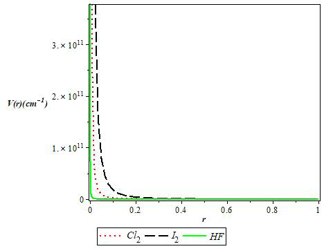
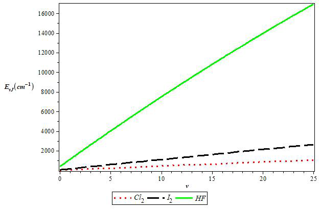
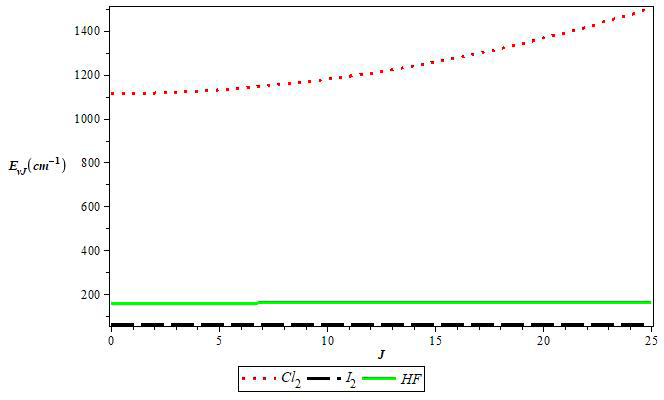
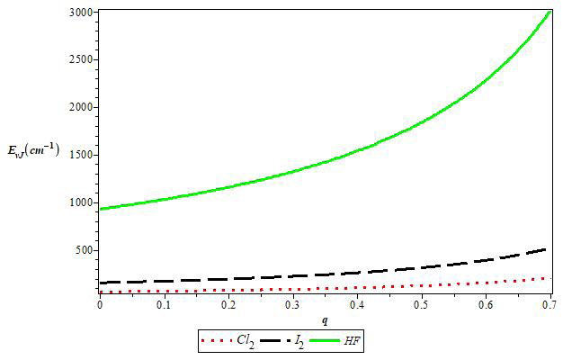
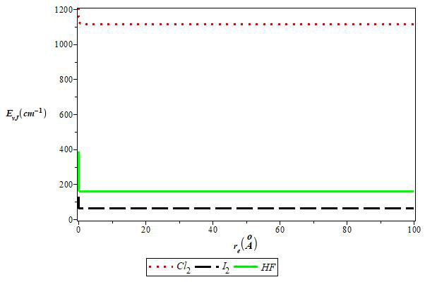
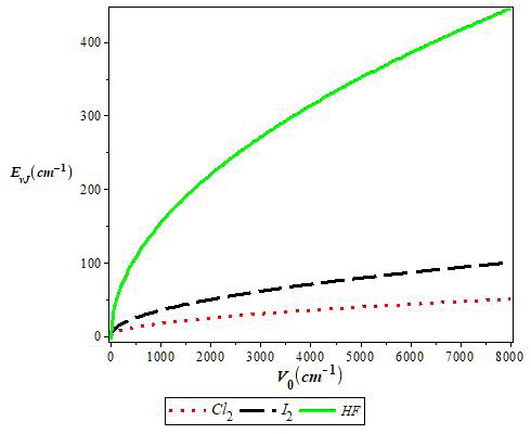
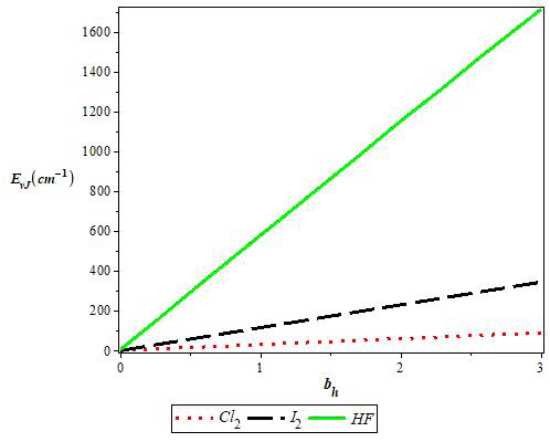
In (Figure 1), we plot the shape of molecular Hua potential for the selected diatomic molecules. The figure gives an insight of the characteristics of the the Hua potential. (Figures 2-7) are various plots showing variation of rotational-vibrational energy against various parameters for the diatomic molecules. A monotonic increase in the energy is seen In (Figure 2) for the molecules as the quantum number, v, and increases. In (Figure 3) the energy is seen to increase with rotational quantum number, J. For Cl2 molecule, the increase is more visible than in I2 and HF molecules. The Cl2 atom appears to shift to higher values than the I2 and HF molecules. (Figure 4) indicates a progressive increase in energy as the deformation parameter, q, and increases. In (Figure 5), the energy of the diatomic molecules is observed to increase as the potential depth, V0, increases. In (Figure 6), we observe an increase in energy of the Hua potential as the parameter, bh, increases for the molecules. In (Figure 7), the energy of the diatomic molecules first decreases as the molecular bond length increases between 0 to 0.04 for the I2 and HF molecules; it then maintains a constant value with increase in the molecular bond length. For the Cl2 molecule, the energy first decreases as the molecular bond length increases between 0 to 0.14.
Conclusion
In this work, we present solutions of Dirac equations with Hua potential energy model using the Formula method. Using the spin symmetry and the Pekeris form of approximation, we evaluated the relativistic rotation- vibrational energy equation for diatomic molecules under the Hua potential. In the nonrelativistic limit, the relativistic energy expression becomes the nonrelativistic rotation- vibrational energy equation. Numerical results are also computed for the selected molecules. The results show considerable agreement with reports in literature. This study can be applied in molecular physics, spectroscopy and other fields of science.
Declaration of Interest
The authors declare that they have no known conflict of interest.
Funding statement
This work did not receive any grant or support from funding agencies.
References
-
Tang HM, Liang GC, Zhang LH, Zhao F, Jia CS, et al. (2014) Diatomic molecule energies of the modified Rosen Morse Potential energy model. Can J Chem 92(4): 341-345.
-
Oluwadare OJ, Oyewumi KJ (2018) Energy spectra and the expectation values of diatomic molecules confined by the shifted Deng-Fan potential. Eur Phys J Plus 133: 422.
-
Yanar H, Aydogdu O, Salti M (2016) Modelling of diatomic molecules. Mol Phys 114: 3134-3142.
-
Hamzavi M, Rajabi AA, Hassanabadi H (2012) The rotation–vibration spectrum of diatomic molecules with the Tietz–Hua rotating oscillator and approximation scheme to the centrifugal term. Mol Phys 110: 389-393.
-
Yanar H, Tas A, Aydogdu O, Salti M(2020) Ro-vibrational energies of CO molecule via improved generalized Pöschl-Teller potential and Pekeris-type approximation. Eur Phys J Plus 135: 292.
-
Polyansky OL, Császár AG, Shirin SV, Zobov NF, Barletta P, et al. (2003) High accuracy ab initio rotation-vibration transitions for water. Science 299(5606): 539-542.
-
Kisoglu HF, Yanar H, Aydogdu O, Salti M (2019) Relativistic spectral bounds for the general molecular potential: Application to a diatomic molecule. J Mol Mod 25(5): 143.
-
Jia CS, He T, Shui ZW (2017) Relativistic rotation- vibrational energies for the CP molecule. Comp Theo Chem 1108: 57-62.
-
Jia CS, Jia Y (2017) Relativistic-rotational vibrational energies for the Cs2 molecule. Eur Phys J D 71: 3.
-
Hassanabadi H, Yazarloo BH, Zarrinkamar S, Solaimani M (2012) Approximate analytical versus numerical solutions of Schrodinger equation under molecular Hua potential. Int J Quant. Chem 112(23): 3706-3710.
-
Hua W (1990) Four-parameter exactly solvable potential for diatomic molecules. Phys Rev A 42(5): 2524-2529.
-
Njoku IJ, Onyenegecha CP, Okereke CJ, Opara AI, Ukewuihe UM, et al. (2021) Approximate solutions of Schrodinger equation and thermodynamic properties with Hua potential. Res Phys 24: 104208.
-
Falaye BJ, Ikhdair SM, Hamzavi M (2015) Formula method for bound state problems. Few-Body Syst 56: 63-78.
-
Tezcan C, Sever R (2009) A general approach for the exact solution of the Schrödinger equation. Int J Theor Phys 48: 337-350.
-
Alhaidari AD, Bahlouli H, Al-Hasan A (2006) Dirac and Klein-Gordon equations with equal scalar and vector potentials. Phys Lett A 349: 87-97.
-
Ikot AN, Okorie US, Osobonye G, Amadi PO, Edet CO, et al. (2020) Superstatistics of Schrodinger equation with pseudo-harmonic potential in external magnetic and Aharanov-Bohm fields. Heliyon 6(4): e03738.
-
Roy AK (2014) Ro‐vibrational studies of diatomic molecules in a shifted Deng–Fan oscillator potential. Int J Quant Chem 114(6): 383-391.
-
Pekeris CL (1934) The Rotation-Vibration Coupling in Diatomic Molecules. Phys Rev 52(2): 110-119.
-
Khodja A, Kadja A, Benamira F, Guechi L (2019) Complete non-relativistic bound state solutions of the Tietz-Wei potential via the path integral approach. Eur Phys J Plus 134: 57.
- Sense, Gravity, Parity & Chirality in Mathematical Physics
- Quantum Lattice Simulations PHYSICS: Microcircuit Particle Formation and Observable Macroscopic Irreversible Time - A Discrete Lagrangian with Cellular Automata Framework
- Quantum Biology from Biomacromolecule to Cell, and Central Dogma Described by Quantum Theory
- Focus, Agility, Speed and Technology (FAST) for Sustainability and Growth
- Square Root Metric Geometry and Pati-Salam Model in Curved Space-Time
- A Simple System Demonstrating the Mpemba Effect in Classical Mechanics