Mathematical Modelling and Simulation of Aluminium Filling in Conical Pipe and Cylindrical Pipe under High Pressure
The desired technology for manufacturing light-weight components from metal alloys mostly aluminum and magnesium alloy is Die casting. High pressure die casting requires the liquid metal to be forced at high speed and pressure through a metal pipe. In our study, we seek to study Aluminum filling under high pressure in two different pipes, cylindrical and conical pipes. Two cases are considered for the cylindrical pipe, when the pipe vertical and when the pipe in inclined at an angle of 450 with the horizontal. The governing equations are obtained and the results are compared. The governing equations are obtained and modeling is done using ANSYS FLUENT. The results show that inclining the cylindrical pipe causes a shift in the oscillations and the inclined pipe has slightly lower amplitude of oscillation implying a greater loss of energy due to the inclination. The inclined cylindrical pipe has higher damping compared to the vertical cylindrical pipe. It is also evident that the conical pipe has higher oscillations than the cylindrical pipe implying a greater loss of energy for the conical cylindrical.
Introduction
Die casting is the process of forcing molten metal under high pressure in metal casting. It is one of the oldest manufacturing process and widely used [1]. The material to be used in the manufacturing is first liquidized by properly heating it in a suitable furnace. The most common molten metal used is aluminum. It then is forced into the cavity of a reusable steel mold (the die) under high pressure [2]. There is an increasing demand for Aluminium die casting worldwide. It is therefore important for the process to be understood in order to make sensible manufacturing choices for the future and thus, there has been a lot of research done on modeling of die casting process to study how different factors affect the process.
Davey and Hindua using a steady state approximation to model the pressure die casting process with the boundary element method [3]. Due to the importance of the temperature on the cavity surfaces on the quality of the component, they were able to use the boundary element method to predict the temperature on the surface. Comparison of the temperatures with other methods yielded good agreement.
Ozlem, et al. [1] performed a computer simulation using commercially available software of a high-pressure die casting of aluminum alloy. The commercial aluminum alloy was Etial 150 (AlSi12Cu) that is used for flange which is a washing machine part. They investigated the mold filling, solidification, temperature distribution, porosity, and velocity of the liquid metal during high-pressure die casting.
The results showed that the model values used in simulations were accurate and were applied in the experimental casting.
Paul, et al. [4] did a computational modelling of thin walled high pressure die casting using Lagrangian method that uses an interpolation kernel of compact support known as smooth particle Hydrodynamics (SPH). The validation of the numerical modelling was done using the water analogue experiment and there was good agreement between the simulated results and the experimental results. In Fu J, Wang K [5], the process of die filling of semi-solid state alloy A356 is simulated. Two non-Newtonian constitutive equations are modeled using the CFD software PROCAST. The results showed that the material the semi-solid metal alloy has a special die filling behavior compared with liquid filling.
In recent years, the advent of mesh free methods has led to the opening of new avenues in numerical computational techniques to follow the physical behaviour of fluid flow. In this paper, we seek to study Aluminium filling in cylindrical and conical pipes.
Methodology
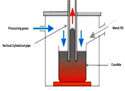
We start by considering a vertical cylindrical pipe made of aluminum titanate immersed in molten aluminum (alloy 226) as shown in Figure 1. The pipe is immersed to a depth of 50mm. The total length of the pipe is 570mm and positive pressure relative to the air on the surface is applied which causes the melt in the pipe to rise to some height h.
We first start by considering the case without dissipation. The total force acting on the liquid column, the kinetic energy and potential energy is calculated. Energy loss due to dissipation is then included by analyzing the causes of dissipation in the system and then incorporating in the energy equation.
The same procedure as in the case of vertical cylindrical pipe is used to study the damped oscillations in an inclined cylindrical pipe. The pipe is immersed at a depth of 50 mm and inclined at an angle of . Positive pressure relative to the air is applied to the liquid surface causing the melt in the pipe to rise to some height h.
Lastly, we consider a vertical conical pipe. It is immersed to the same depth as the cylindrical vertical pipe, i.e to a depth of 50mm and the same methodology will be followed as that of the vertical cylindrical pipe.
Governing Equations
Case I: Vertical Cylindrical Pipe
We first consider a case without dissipation. The total force acting on the liquid column, the kinetic energy and potential energy is calculated. The next step is then to analyze the causes of dissipation in the system and then incorporate them in the energy equation.
Total Energy: The potential energy is obtained by considering
the force acting in the liquid column and integrating it by
taking the potential force
$$ E _ {p} = 0 $$
for h = 0 to get the potential
energy as:
$$ E _ {p} = \frac {1}{2} \rho g A h ^ {2} \tag {1} $$
The kinetic energy is given as:
$$ E _ {k} = \frac {1}{2} m v ^ {2} = \frac {1}{2} \rho A (h + H) \dot {h} ^ {2} \tag {2} $$ The total sum of energy in the column is obtained by summing up equations 1 and 2. The differentiated energy together with the 1st principle of thermodynamics gives the balance of energy equation. This gives the energy without dissipation as:
$$ \frac {1}{2} \rho A \left(2 (h + H)\right) \dot {h} \ddot {h} + \dot {h} \dot {h} ^ {2} + 2 g h \dot {h}) = p A \dot {h} $$ (3) To get the total energy equation, energy lost due to dissipation is analyzed and incorporated into equation 3. The losses in the pipe are due to friction on account of the roughness of the wall and also due the singular pressure loss at the entrance or exit of the pipe if liquid rises or if liquid goes down respectively. The energy loss due to friction can be written as:
w W dE p V = ∆ (4)
The pressure loss due to friction as given by Darcy formula is given as
$$\Delta p_w = \frac{\rho f v^2}{2 D_h},$$ which can be written as:
$$\Delta p_w = \frac{\rho f}{2 D_h} (h + H) \dot{h}^2 = \frac{\rho f H}{2 D_h} \left( \frac{h}{H} + 1 \right) \dot{h}^2 = \frac{1}{2} \rho k_w \left( \frac{h}{H} + 1 \right) \dot{h}^2$$
where $k_w = \frac{f h}{D}$ Thus,
$$d E_w = \frac{1}{2} k_w \rho A \left( \frac{h}{H} + 1 \right) \dot{h}^2 |\dot{h}|$$
The singular pressure loss is given as
$$d E_w = \frac{1}{2} k_w \rho \dot{h}^2 |\dot{h}|$$
Equations 5 and 6 are included in Equation 3 to obtain the final equation:
$$\left( (h + H) \ddot{h} + \frac{\dot{h}^2}{2} + g h \right) + \frac{1}{2} \left( k_E + k_w \left( \frac{h}{H} + 1 \right) \dot{h} \right) |\dot{h}| = \frac{p(t)}{\rho}$$
**Case II: Inclined Cylindrical Pipe at an Angle**
Just as is the case with the vertical pipe, the total force acting on the liquid column, the kinetic energy and potential energy is calculated and then the causes of dissipation in the system are analyzed and incorporated in the energy equation.
Total Energy: The total energy is obtained, like in the previous case, by adding the kinetic and potential energy. We also analyze the energy losses due to dissipation and included it to get the governing energy equation. Using the potential energy formula $d E_p = m g d Z$ and considering that $l = \frac{h + H}{\sin(\theta)}$ and $l' = \frac{h}{\sin(\theta)}$, the potential energy in the tube will be given by:
$$E_p = \int m g d Z = \int \rho g A l' d Z = \frac{\rho g A}{\sin(\theta)} \int_0^h z d Z = \frac{1}{2} \rho g A \frac{h^2}{\sin(\theta)}$$
By using the kinetic energy formula and length $l = \frac{h + H}{\sin(\theta)}$ and $l' = \frac{h}{\sin(\theta)}$, for the inclined vertical pipe, the kinetic energy formula is given by:
$$E_k = \frac{1}{2} \rho A \frac{h + H}{\sin(\theta)} \left( \frac{h}{\sin(\theta)} \right)^2$$
Summing up the potential and kinetic energy, the total sum of energy is given by:
$$E = \frac{1}{2} \rho A \left( g \frac{h^2}{\sin(\theta)} + \frac{(h + H) h^2}{\sin^3(\theta)} \right)$$
Differentiating the energy equation, we obtain
$$\dot{E} = \frac{1}{2} \rho A \left( 2 g h \dot{h} + \frac{\dot{h} h^2}{\sin^2(\theta)} + \frac{2 (h + H) h \dot{h}}{\sin^3(\theta)} \right)$$
To get the governing energy equation, we need to analyze and incorporate energy losses due to dissipation into equation 11. To obtain the loss due to friction, $|\dot{V}|$ is replaced with $|\dot{l}|$ into equation 5 and use Darcy's formula.
Thus the energy loss due to friction is given as:
$$E_w = \frac{\rho \lambda A (h + H) h^2 |\dot{l}|}{2 D_h \sin^4(\theta)} = \frac{\rho \lambda \pi r^2 H \left( 1 + \frac{h}{H} \right) h^2 |\dot{l}|}{4 r \sin^4(\theta)} = \rho A k_w \left( 1 + \frac{h}{H} \right) h^2 |\dot{l}| 2 \sin^4(\theta)$$
With $k_w = \frac{\lambda H}{2 r}$
Similarly, the singular pressure loss at the entrance of the pipe is obtained by replacing $|\dot{V}|$ with $|\dot{l}|$ in equation 7 to obtain:
$$\Delta p_E = \frac{1}{2} k_E v^2 = \frac{1}{2} \rho k_E l^2 = \frac{1}{2} \rho k_E \frac{h^2}{\sin^2(\theta)}$$
The final equation energy equation with dissipation is obtained by incorporation equations 12 and 13 into equation 11 and simplifying to get:
$$\left( g h + \frac{\dot{h}^2}{2 \sin^2(\theta)} + \frac{(h + H) h}{2 \sin^2(\theta)} + k_E \frac{\dot{h} |\dot{l}|}{2 \sin^2(\theta)} \right) + \left( k_w \left( 1 + \frac{h}{H} \right) \frac{\dot{h} |\dot{l}|}{2 \sin^2(\theta)} + k_E \frac{\dot{h} |\dot{l}|}{2 \sin^2(\theta)} \right) = \frac{p(t)}{\rho}$$
Case III: Vertical Conical Pipe
The same procedure is done for the vertical conical pipe as was in the previous cases. To get the potential energy, we use the potential energy formula and the radius, $r = R_0 + \frac{z}{\tan \alpha}$
to obtain:
$$ E _ {p} = \rho g \pi \left(\frac {R _ {o} ^ {2} h ^ {2}}{2} + \frac {2 R _ {o} h ^ {3}}{3 \tan \alpha} + \frac {h ^ {4}}{4 \tan^ {2} \alpha}\right) $$
2 2 3 4
2 2 2 3tan 4tan (15)
The Kinetic energy is obtained by getting the kinetic of a
small region z, then integrating over the whole region from
-H to h. We get a function for the velocity of the small region
v(z) using the flow rate Q equation
$$ Q = \frac {d v}{d t}. $$ The volume is given as:
( ) ( ) 2 2 2 3 3 2 0 tan tan 3tan
$$ = \pi \int_ {- H} ^ {h} \left(R _ {o} + \frac {z}{\tan \alpha}\right) ^ {2} d z = \pi \left[ R _ {0} ^ {2} (h + H) + \frac {R _ {o} \left(h ^ {2} - H ^ {2}\right)}{\tan \alpha} + \frac {h ^ {3} + H ^ {3}}{3 \tan \alpha} \right] $$ $$ V = \pi \int_ {- H} ^ {h} \left(R _ {o} + \frac {z}{\tan \alpha}\right) ^ {2} d z = \pi \left[ R _ {0} ^ {2} (h + H) + \frac {R _ {o} \left(h ^ {2} - H ^ {2}\right)}{\tan \alpha} + \frac {h ^ {3} + H ^ {3}}{3 \tan \alpha} \right] $$ h o (16) To obtain the velocity equation, equation 14 is first differentiated to get the flow rate Q and the result divided by the cross-sectional area and then
2 $$ d V = A (z) d z = \pi \left(R _ {o} + \frac {z}{\tan \alpha}\right) ^ {2} d z $$ is replaced into the result, ( ) integrated and simplified to obtain the kinetic energy in the whole pipe as:
$$ = \frac {1}{2} \rho \pi \left(R _ {0} + \frac {h}{\tan \alpha}\right) ^ {3} \left(\frac {h + H}{R _ {o} + \frac {h}{\tan \alpha}}\right) h $$
3 2 0 1 2 tan tan h h H E R h h R ρπ α α (17)
K
o The total energy is obtained by summing Equations 14 and 16 and differentiating the result to obtain and using the 1st principle of thermodynamics dE pdv = . The total energy equation is thus given as:
$$ \dot {h} + \frac {3}{2} \left(\frac {h + H}{R _ {o} - \frac {H}{\tan \alpha}}\right) \left(\frac {\dot {h} ^ {2}}{\tan \alpha}\right) + \frac {1}{2} \left(R _ {0} + \frac {h}{\tan \alpha}\right) \left(\frac {\dot {h} ^ {2} + 2 (h + H) \dot {h}}{R _ {0} - \frac {H}{\tan \alpha}}\right) = \frac {1}{2} $$ ¨ 2 2 ( )
2 3 1 2 tan 2 tan tan tan o h h H h h H h h p gh R H H R R α α ρ α α
0
0 (18) The possible energy losses due to dissipation are analyzed and incorporated into Equation 17.
The energy loss due to friction is obtained, 2 3 2 0 2 2 1 1 2 tan tan o w w R h h h dE k h R H ρ π α α = + + + and the singular pressure loss, 2 2 1 ( ) 2 tan E E o h dE k R h h ρπ α = + is incorporated into equation 17 and simplified to get the final energy equation:
$$ \begin{array}{l} i + \frac {3}{2} \left(\frac {h + H}{R _ {o} - \frac {H}{\tan \alpha}}\right) \left(\frac {\dot {h} ^ {2}}{\tan \alpha}\right) + \frac {1}{2} \left(R _ {0} + \frac {h}{\tan \alpha}\right) \left(\frac {\dot {h} ^ {2} + 2 (h + H) \dot {h}}{R _ {0} - \frac {H}{\tan \alpha}}\right) \\ + \frac {1}{2} k _ {w} \left(1 + \frac {h}{H}\right) \dot {h} | \dot {h} | + \frac {1}{2} k _ {E} \dot {h} | \dot {h} | = \frac {p}{\rho} \\ \end{array} $$ ¨ 2 2 ( )
2 3 1 2 tan 2 tan tan tan 1 1 1 2 2
h h H h h H h h gh R H H R R
0 α α α α
0 o h p k h h k h h H
w E
ρ (19)
Validation
To validate if the equations are correct, we consider equations the total energy equations, equations 8, 14 and 19. For equation 8, we consider a steady state case, thus $$ h = \dot {h} = 0 $$
and considering no loss due to dissipation, we obtain from
equation 8: ( ) ( ) $$ g h = \frac {p (t)}{A} \Rightarrow h _ {0} = \frac {p (t)}{\rho g} $$
To check for the inclined pipe, for it to be considered vertical, sin θ must be equated to
900. The length l
$$ l = h + H; $$
and equation 14 thus reduces to
equation 8. To check the total energy equation for the conical
pipe, we consider the case of cylindrical pipe in which case
90 α =
οand the radius will be constant throughout the pipe.
Thus, Equation 19 will reduce to that of a cylindrical pipe
when 90 α =
οsince any term consisting of tan α in the
denominator will tend to zero. Equations 8, 14 and 19vwere
plotted for values of sin( )
90 θ =
οand tan ( )
$$ (\alpha) = 9 0 ^ {\circ}. F r o m $$
Figure 2, it is apparent that the two equations 14 and 19 both
reduce to equation 8.
![Figure 2: Graph of h[t] for the vertical cylindrical, inclined cylindrical and conical pipe as a function of time for kw = 0.09375, kE = 0.9054, H = 50mm, ρ = 2460kg/m3, 0 tan 90 á = , 0 sin 90 è = with a pressure jump.](/fulltextimages/9092/fig_2.png)
Numerical Modelling
Case of Cylindrical Pipe
We begin the discussion of the numerical results for the conical pipe inclined at an angle. The modeling was done in Ansys Fluent in which case we used a pressure-based, steady solver. The model used was k-epsilon, standard and enhanced wall treatment. Using Bernoulli’s equation, the kinetic energy was calculated using computed pressure and velocity values from Ansys Fluent. The Bernoulli equation gives $$ p _ {1} + \frac {1}{2} \rho v _ {1} ^ {2} = p _ {2} + \frac {1}{2} \rho v _ {2} ^ {2} $$ and since 2 2 1 2 v v < it implies that 2 1v can be neglected. This leads to ( ) 1 2 2 2 2 P P v ρ − = + For a real fluid, we have $$ p _ {1} + \frac {1}{2} \rho v _ {1} ^ {2} = p _ {2} + \frac {1}{2} \rho u _ {2} ^ {2} + \frac {1}{2} k _ {E} \rho v _ {2} ^ {2} \tag {20} $$ Neglecting 2 1v in Eqn 20, calculating KE, we obtain
1 2 E p P u k v
2 1 2 2 ρ $$ = \frac {p _ {1} - P _ {2} - 1}{o v ^ {2}} $$
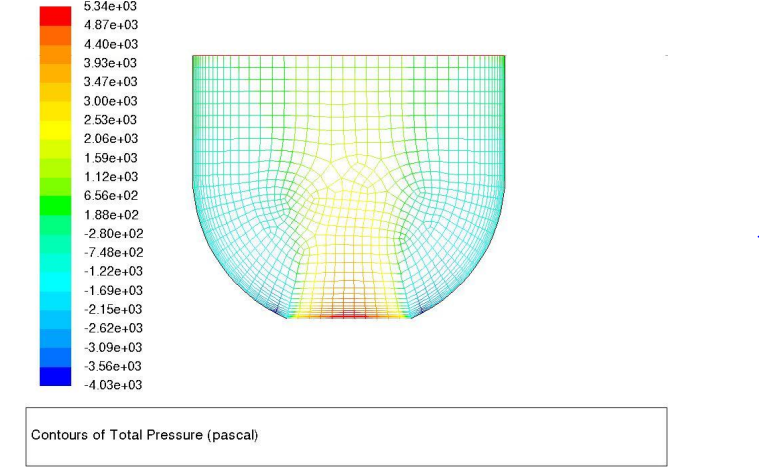
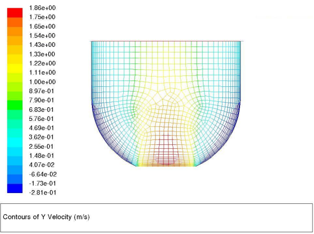
2 2 ρ From the simulation in Fluent, for the cylindrical pipe $$ v _ {2} ^ {2} = + \frac {2 (7 3 7 7 . 2 4 3 - 8 1 5 . 6 4 1 3)}{2 4 6 0} = 5. 3 3 2 8 $$ $$ k _ {E} = 1 - \frac {0 . 7 0 9 3 2 9 2 ^ {2}}{5 . 3 3 2 8 3} $$ The contours of the total pressure and the Y-velocity are plotted (Figure 3 & 4).
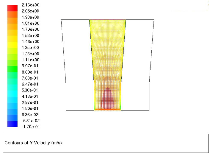
Case of Conical Pipe
The same procedure was done for the case of the conical, the was calculated.
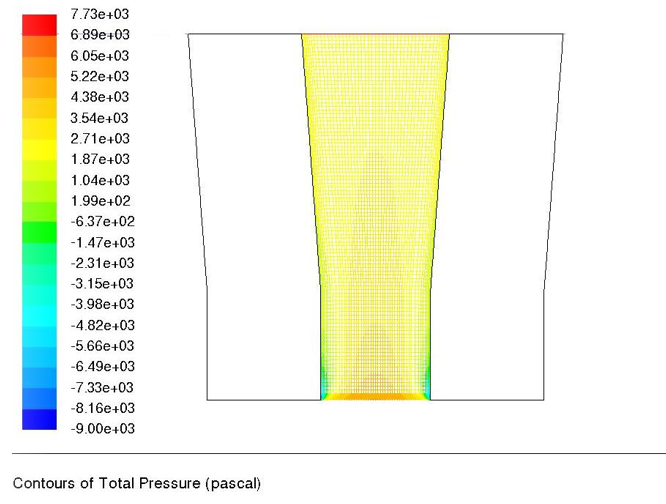
For the simulation in Fluent, for the conical pipe $$ v _ {2} ^ {2} = \frac {2 (7 2 5 2 . 4 1 0 8 - 2 1 9 0 . 4 4 9 5)}{2 4 6 0} = 4. 1 1 5 4 $$ $$ k _ {E} = 1 - \frac {1 . 3 3 9 8 ^ {2}}{4 . 1 1 5 4} = 0. 3 $$ The contours of total pressure and Y-velocity for the conical pipe were plotted (Figures 5 & 6).
Piecewise Function
A piecewise function was used to define the pressure. The pressure was given as a linear function as
0, 1 ( ) 817.77 817.77, 1 10 7360, 10
t p t t t t $$ () = \left\{ \begin{array}{l l} 0, & t < 1 \\ 8 1 7. 7 7 t - 8 1 7. 7 7, & 1 < t < 1 \\ 7 3 6 0, & t > 1 0 \end{array} \right. $$ Initially we had used a jump in pressure given as
0, 1 ( ) 7360 1
t p t t $$ ) = \left\{ \begin{array}{l l} 0, & t < 1 \\ 7 3 6 0 & t < 1 \end{array} \right. $$ To compare the effects of the different pressure function on the height function equation, the graph was plotted (Figure 7).
![Figure 7: Graph of h[t] as a function of time for kw = 0.09375, kE = 0.9054, H = 50mm, 3 2460 / kg m ρ = for different pressure functions.](/fulltextimages/9092/fig_7.png)
Results and Conclusion
To compare vertical cylindrical pipe and conical pipe,
we use the
ek obtained from the numerical modeling and
the linear pressure function and plot the graph of height
h(t) as a function of time t. Figure 8 was plotted for the
different values of
$$ k _ {E} \left(k _ {E} = 0. 9 8 9 5 f\right) $$
for cylindrical pipe and
$$ k _ {E} = 0. 1 0 6 0 $$
for conical pipe).
![Figure 8: Graph of h[t] as a function of time for](/fulltextimages/9092/fig_8.png)
$$ k _ {w} = 0. 0 9 3 7 5 $$
and (cylindrical pipe) and
$$ k _ {E} = 0. 1 0 6 0 $$
(Conical pipe) with $$ H = 5 0 m m, R = 0. 0 1 0 8 m, p = \frac {2 4 6 0 k g}{m ^ {3}} $$ , and at t = 0, p = 0, at t = 10, p = 7360Pa It is clear that, the conical pipe has greater oscillations than the cylindrical pipe.
To compare the vertical cylindrical and inclined pipe, Figure 9 was plotted for the same E k and w k values. It is clear that the inclined pipe has higher oscillations than the vertical cylindrical pipe.
![Figure 9: Graph of h[t] as a function of time plotted for the vertical and inclined cylindrical pipe with](/fulltextimages/9092/fig_9.png)
3 2460 0.09375, 1, 50 , w E kg k k H mm p m = = = = and at
0, 0, 10, 7360 t p at t p pa = = = = .
For the case where there is no dissipation ($k_E = k_w = 0$) for the vertical and inclined cylindrical pipe, the fluid will oscillate in the pipe indefinitely since there is no energy lost either through friction or at the entry. For the case of dissipation, the higher the energy lost, the higher the amount of damping of the oscillation. It is evident from Figure 9 that inclining the cylindrical pipe causes a shift in the oscillations and the inclined pipe has slightly lower amplitude of oscillation implying a greater loss of energy due to the inclination. It is evident from the graph that the conical pipe has higher oscillations than the cylindrical pipe implying a greater loss of energy for the conical cylindrical.
References
-
Boydak O, Savas M, Ekici B (2016) A numerical and experimental investigation of a high-pressure die-casting aluminium alloy. International Journal of Metal Casting 10(1): 56-69.
-
Dalquist S, Gutowski T (2004) Life Cycle Analysis of Conventional Manufacturing Techniques. Sand Casting. Volume 2, Massachusetts Institute of Technology, Cambridge, USA, pp: 1-13.
-
Davey K, Hinduja S (1990) Modelling the pressure die casting process with the boundary element method. Steady State Approximation 30(7): 1275-1299.
-
Cleary PW, Savage G, Ha J, Prakash M (2014) Flow analysis and validation of numerical modelling for a thin walled high pressure die casting using SPH. Computational Partical Mechanics 1: 229-243.
-
Fu J, Wang K (2014) Modelling and simulation of die casting process for A356 semi-solid alloy. Proceedings Engineering 81: 1565-1570.
- Sense, Gravity, Parity & Chirality in Mathematical Physics
- Quantum Lattice Simulations PHYSICS: Microcircuit Particle Formation and Observable Macroscopic Irreversible Time - A Discrete Lagrangian with Cellular Automata Framework
- Quantum Biology from Biomacromolecule to Cell, and Central Dogma Described by Quantum Theory
- Focus, Agility, Speed and Technology (FAST) for Sustainability and Growth
- Square Root Metric Geometry and Pati-Salam Model in Curved Space-Time
- A Simple System Demonstrating the Mpemba Effect in Classical Mechanics