Overview of Optical Technology for Aerosols Characterization

Basis of Photometric Measurements in the Visible Spectrum

Indicators that help us to characterize radiation is the wavelength ($\lambda$) and the frequency ($\nu$), both being inverse equivalents. Radiation is emitted by matter when an electron falls to a lower energy level. This energy difference between the levels ($\Delta \varepsilon$) is related to the frequency of the radiation emitted directly and proportionally to Planck’s constant ($h$) as can be seen in Equation 1, which also applies to the absorption of a photon by a molecule. In this sense, a molecule can absorb radiation whose wavelength corresponds to the difference between two of its energy levels. This causes different molecules to efficiently absorb different wavelengths radiation. The mechanics within the phenomenon of molecular absorption of radiation can be explained by quantum chemistry, where the geometry of the molecules and the distribution of charges are the parameters to consider.

$$\Delta \varepsilon = h \nu = \frac{h c}{\lambda} \quad (1)$$

A photometer is an instrument that makes use of the absorption by aerosols in the optical path of radiation as transduction in its measurements. This can be from the incident solar radiation measured in an entire atmospheric column or a beam of light with a finite path determined on a laboratory scale. One of the parameters measured is the Aerosol Optical Depth (AOD), which is the integrated extinction coefficient of radiation at a given wavelength over the entire optical path [1]. In atmospheric studies, the AOD is a columnar property that is influenced by local and mesoscale processes, and many researchers have used it to characterize regional pollution [2]. In this domain, AOD can be measured with surface sun photometers and can also be derived from satellite measurements of Earth-reflected radiation [3].

Solar photometers under regulation use interferential filters and photo detectors, but this is a technology not affordable for institutions with limited resources. An alternative is given by photometers based on LED (light emitting diode) technology, which represent a low-cost alternative that allows acquiring valid measurements of AOD, especially in regions not covered by official programs. Direct measurements from a LED photometer are used to calculate the AOD at each wavelength based on the Lambert-Beer law applied to the atmosphere, considering that the total atmospheric optical thickness depends only on the dissipation of light caused by molecules known as Rayleigh scattering, by molecules of ozone ($O_3$) and aerosols (Equation 2).

$$I(\lambda) = Io(\lambda) \exp \left[ -m \left( \tau_a + \tau_{03} + \tau_r \right) \right]$$

Where $I(\lambda)$ is the intensity of the sunlight received on the surface for a given wavelength, $Io(\lambda)$ the intensity of sunlight outside the atmosphere, $m$ is the coefficient of the air mass that the light passes through until it reaches the surface [4], $\tau_a$ is the coefficient of aerosol transparency also known as AOD, and $\tau_{03}$ is the coefficient of ozone transparency. $\tau_r$ (Equation 3) is the transparency coefficient of Rayleigh scattering, proportional to the ratio of the measured atmospheric pressure $P$ at the point of observation and the pressure at sea level $p_0$ [5].

$$\tau_r = a_r \frac{P}{p_0}$$

$a_r$ is the contribution to the optical thickness of molecular Rayleigh light scattering in the atmosphere. The aerosol transparency coefficient can be calculated from a value of $N$ directly proportional to the intensity of light recorded by the photometer, as indicates Equation 4.

$$\tau_a = \frac{\ln \left( N_0 \left[ \frac{r_0}{r} \right]^2 \right) - \ln(N)}{m} - a_r \frac{P}{p_0} - \tau_{03}$$

$N_0$ is the value that the photometer would record for measurement of light intensity outside the atmosphere at a distance from the Sun $r_0$ equal to 1 AU (astronomical unit) [6]. The calculation of the AOD requires the distance to the Sun $r$ in AU for the time the measurement was taken (which is calculated based on the geographical coordinates of the measurement site and the day of the year).

The Ångstrom coefficient ($\alpha$) (Equation 5) is a quantity sensitive to the size distribution of aerosols and is calculated from the spectral dependence of AOD in logarithmic space [7]. This coefficient turns out to be inversely proportional to the mean square radius of the particles, varying between 4 (for small particles) and 0 (for large particles) [8].

$$\alpha = \frac{\ln \left( \frac{\tau_a}{\tau_{03}} \right)}{\ln \left( \frac{\lambda_1}{\lambda_2} \right)}$$

More information can be provided by the relationship between the Ångstrom coefficient and the AOD. A graph between these two variables allows identifying the main groups of aerosols present and their characteristics according to climatic classification [9]. Aerosols can be classified according to the size of the particles and their characteristics of light absorption. The classification gives us an idea of the main types of aerosols present in a sample and we can trace their origin and behavior over time, but there are different approaches to doing it.

Coherent Light Scattering Measurement Basis

Leaving molecular gases aside for a moment, there are particles in the atmosphere and in different natural and artificial subsystems whose sizes range from a few nanometers to about 100 $\mu$m, and which can also be characterized from optical approaches. As an example, photochemically produced aerosols usually have sizes less than 1 $\mu$m, while dust, pollen, or salt particles have sizes greater than that threshold. As premises for the mathematical development, the particles are considered spherical and made up of an integer number of molecules or monomers (the smallest being the one made up of 2 molecules).

The distribution of aerosols present in a sample can be characterized by the concentration number ($N_r$) in each size range, which is the concentration of particles containing the molecules. Each range is a discrete interval of one particle size division. The size distribution can also be described by the cumulative distribution, which is defined as the concentration of particles that are less than or equal to a certain size. The last value of the cumulative distribution represents the total concentration number.

Optical techniques for measuring particulate matter (PM) are based on light scattering, making use of a low-power source, either an LED or a laser, where the particles that are collected scatter the light (in a phenomenon set of reflection, refraction, and diffraction) that is measured by a photodetector in the device. This detector is usually a bipolar transistor called phototransistor which is able to alter the current flowing between its emitter and collector according to the intensity of the light received. The concentration of particles is proportional to the intensity of scattered light and distribution is assumed density and particle size determined. Most of these sensors usually have a mini-cooler to force air circulation through the chamber sampling.

Optical applications for PM measurement employ two techniques. On the one hand, nephelometry (which measures the light scattering of particles from a set of aerosols) and, on the other hand, optical particle counting (which measures the size of the particles and the number of individual particles). The actual particle size detection limit of these sensors is usually greater than 3 μm. Although they have advantages such as negligible response times (they depend on the light transfer within the chamber and the rate of electron transport in the circuit) and have no interference equivalents, its reported performance in the literature is somewhat heterogeneous [10, 11] and may depend on the type of particle sensor used (of which there is a great variety on the market).

All PM low-cost sensors (LSC) have their problems when it comes to distributing particle sizes in bins and, in general, calibration/validation works normally use PM${2.5}$ concentrations (particle sizes less than 2.5 μm) as a reference because it is the most reliable in these instruments [11]. This is based on the fact that LCSs only capture a very small fraction of aerosol particles and therefore rely heavily on statistics and extrapolation. The count number density of the PM${10}$ fraction (particle sizes less than 10 μm) of typical aerosols is extremely low; therefore, that fraction cannot be measured directly with these sensors.

It is necessary to delve into some other concepts and theories that are used when characterizing the presence of particles in the air based on their interaction with light, for a deepest PM LCS assessment. The intensity of the light scattered by aerosols is a function of $\lambda$, the angle of scattering ($\theta$) measured concerning the direction of the incident light, the particle diameter ($D_p$), and the relative refractive index ($n$) between the particle and the medium. The relationship between $D_p$ and $\lambda$ indicates the dispersion regime:

• If the particle size is similar to the wavelength of the incident light, we are in the Mie regime for scattering (the most common case for aerosols atmospheric).
• If the size is much smaller than the wavelength, the dispersion is explained through the Rayleigh regime. This component is what is subtracted in Equation 4 to determine the extinction of light in a photometric measurement.
• If the particle size is much larger than the wavelength of light, then a simplified geometric dispersion is enough.

Mie’s theory [12] predicts a dispersion pattern based on the relationship between the intensity of the light and the angle of detection, with which a particle size distribution can be determinate. To do this, some assumptions must be made [13]:

• Light is monochromatic and consists of plane waves.
• The particles are spherical and isotropic.
• Both absorption and scattering of light are considered.
• Light scattered from one particle to another is negligible.
• The scattering characteristics are independent of the motion of the particles.
• Quantum effects are not considered.

The mathematical formalism of Mie’s theory is out of the scopes of this review, but we can say that is an elegant solution to Maxwell’s equations, which allows the calculation of electromagnetic fields for spherical objects. This is suitable to study the scattering of light by particles, giving as results the Mie resonances within information about the strength of scatter according to particle sizes.

A laser spectrometer for aerosol measurement (the mechanism used by PM LCS) works by collimating a beam of light perpendicular to the incoming airflow to the detection chamber. When the laser insides on a particle the light is scattered, and a fraction of it is collected at a given angle by a detector. Following Mie’s theory, the amplitude of each measured pulse correlates with the size of the particles. Each pulse is counted and assigned to one of the standardized bins (ranges) of sizes [13].

To modelling the distribution of aerosols present in an air sample, it can be considered as composed of a sum of $i$ lognormal modes, as indicated in Equation 6 [13]:

$$\frac{dN}{d\log(D_p)} = \sum_{i=1}^{n} \frac{N_i}{\sqrt{2\pi} \log(\sigma_i)} \exp \left( -\frac{\left( \log(D_p) - \log(\bar{D}_{p,i}) \right)^2}{2\log^2(\sigma_i)} \right)$$

Where $N$ is the number of particles (then $N_i$ is called the concentration number of each mode $i$ (i.e. number of particles per cm$^3$), $\sigma_i$ the standard deviation diameter (variety of particle size) and $\bar{D}_p$ is the geometric mean of the diameter particle size (the median of the size distribution for each mode).

Likewise, some characteristics that affect the optical properties must be determined to finish defining a particle distribution mode. These are the hygroscopic growth factor (f(RH)), the particle density (ρ), and the complex refractive index (mi) (whose real part indicates the ratio between the speed of light in the medium and in a vacuum, and whose imaginary part corresponds to the coefficient of light extinction).

The probability distribution function is given by the final sum of all the modes in Equation 6, and is also called the concentration number function since the area under the curve of the graph of dN/dlog(Dp) vs Dp is equal to the number of overall concentration.

By multiplying the distribution in Equation 6 by the particle volume simplified to a sphere, the volumetric distribution is obtained. If this distribution is integrated between two particle sizes the volumetric cumulative distribution function is deducted, and its product with the density allows us to estimate the mass load of aerosols per volume unit, which we call particulate matter (PM in µg/m3) between chosen diameters (Equation 7). For example, PM2.5 arises from integrating the volumetric distribution between diameters 0 and 2.5 µm and multiplying by the density ρ.

$$ P M = \rho \frac {\pi}{6} \int_ {D _ {\min }} ^ {D _ {\max }} D _ {p} ^ {3} n _ {N} \left(D _ {p}\right) d D _ {p} \tag {7} $$ ( ) 3 6 D max min

Overview of the State of the Art in Photometric Measurements for the Characterization of Aerosols

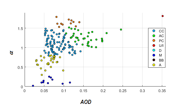
This section is designated on the characterization of sizes and composition of aerosols based on photometric measurements of the atmosphere through satellite measurements or surface instruments. There are different aerosol classification schemes based on optical properties, the most widely used being the graphical method of AOD vs α [14, 15, 16]. In this way, aerosols are classified based on their absorption capacity at different wavelengths and their size ranges. Figure 1 shows an example with own measurements made in Buenos Aires, Argentina, with a low- cost sun photometer (CALITOO from TENUM, based on LED technology). Absorption was measured at 440 nm, and α was calculated from the wavelengths of 440 nm and 675 nm.

Click to enlarge

Chen, et al. [17] compared four different classification schemes using ground and satellite observations and found that each was consistent with the references and with the others. These schemes use three variables, AOD, α, and single scattering albedo (SSA), which is the ratio of the scattering component to the total extinction of light at a given wavelength. This indicates that there is no universally accepted scheme, and the preference between them is often dependent on geographic location.

Schmeiser, et al. [18] compared three methods to estimate dominant aerosol types at 24 different sites. The first consisted of plotting α vs. the Scattering Armstrong Exponent (using the SSA for its calculation), the second expands the approach by introducing multivariate clustering grouping stations with similar characteristics, and the third was based on an analysis of back trajectories of air masses. All three methods were robust and the general approach helped to reduce ambiguity when classifying aerosols with optical methods. It is beneficial in the pursuit of a more complete interpretation of results the use of comprehensive classification methods that consider characteristics of the locations and influences at the regional level.

Zhang, et al. [19] combined optical property measurements from the MODIS satellite instrument with a geographically weighted regression (GWR) to identify spatial relationships of AOD in a region of China. In this way, they found contamination hotspots, and developed a spatial prediction method for AOD from the perspective of land- use change, which represents a valuable tool when making decisions. The distribution of aerosols at the local level also depends on local characteristics, such as different land uses and pollution sources.

Valentini, et al. [20] combined aerosol optical properties, chemical composition, and size distribution to characterize the physical-chemistry of aerosols in Rome, Italy. In this way, they designed a classification model that allows for characterizing different episodes of aerosols. This work reminds us that an interdisciplinary approach is essential to achieve a better understanding of the problem at hand.

An interesting approach is to implement machine learning techniques in order to extract more information from the optical property data. Choy, et al. [21] developed a new aerosol classification method by applying a random forest model with optical property data. The results were compared with a model of AOD vs SSA and showed that the model manages to predict correctly with a good sensitivity towards non-spherical particles. This paper is the first attempt (to the best of my knowledge) to model aerosol classification based on learning optical properties, instead of plotting thresholds on the values ​of the variables or using a clustering technique.

Overview of the State of the Art in Particle Measurements through Light Scattering

Alfano, et al. [22] presented a very complete review of different low-cost PM sensors, with light scattering technology. They conducted a survey of the literature on sensor calibrations, different types of uses, and their performance in characterizing particle size distributions. They concluded that, of the 50 models presented, most have good performance compared to gravimetric equipment under regulation. However, calibration and a periodic inspection are crucial. This indicates that low-cost optical sensors still have a long way to go, but they can provide valuable information in places where there are no regulated measurements.

Kuula, et al. [23] investigated the size selectivity of different particulate optical sensors. They found that none of the models can detect the ranges stated by the manufacturers. For this reason, the limitations of this type of sensor must be taken into account prior to its use and when drawing conclusions about its measurements.

Hagan and Kroll [24] presented a novel framework and open-source Python package to evaluate the capabilities of different optical sensors when measuring particle size distributions and mass concentration of aerosols. They concluded that the uncertainties in the measurements are dependent on the type of sensor technology (nephelometer or particle counter), the specific manufacturing parameters, and the equivalence between the aerosols used to calibrate the sensors and those to which they are later exposed during the measurements. This package is a very interesting resource as a complement to characterize a light scattering sensor.

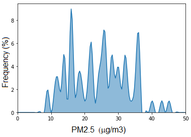
Figure 2 shows a frequency distribution of PM2.5 concentrations for own measurements made with an optical sensor (PMS5003 from Plantower) in Buenos Aires, Argentina. The analyzed data, as well as the figure, show how noisy the signals from these sensors can be. That is why it is very important to study the limitations of sensing in laboratory, carry out throughout calibrations with reference instruments, and draw conclusions from their data with great caution.

Click to enlarge