Analysis of Aluminium Filling in Cylindrical Pipe under High Pressure by Experiment and Mathematical Modelling
The preferred method for producing lightweight metal components, mainly from aluminum and magnesium alloys, is through high pressure die casting. This process involves rapidly and forcibly injecting liquid metal into a metal mold under high pressure. Our study aims to compare results obtained from the numerical modelling of the filling of aluminum under high pressure with the experimental results. Two different cylindrical pipes are used. The results indicate for imposed values of KE = 14 and KW = 60 for pipe 1(Dentry/Drp=40/40) and pipe 2 (Dentry/Drp=16/40) respectively, the mathematical model with the same initial conditions gives some results which are close to the experimental data. The results also indicate that pipe 2 is damped faster than pipe and this is due to the singular pressure loss at the entry.
Introduction
Die casting is the process of forcing molten metal under high pressure in metal casting. It is one of the oldest manufacturing processes and widely used [1]. It is an effective method for mass-producing metallic parts and structures with complex shapes and geometries. It is widely utilized in industries such as the automotive sector, where productivity is a crucial factor in the choice of manufacturing process for large-scale production. It is suitable for large- scale production of components with low per-part costs [2].
The process of die casting involves injecting molten metal into a reusable steel mold (the die) using high pressure. A metal is heated in a furnace until it reaches a liquid state, after which it is forced into a mold [3]. The demand for aluminum die casting continues to grow thus making it crucial to understand the process in order to make informed manufacturing decisions. There has been extensive research into modeling the die casting process, examining how different factors impact it.
Paul, et al. [4] employed the Lagrangian method and the smooth particle hydrodynamics (SPH) interpolation kernel to perform a computational modeling of thin-walled high- pressure die casting. The numerical modeling was validated using a water analogue experiment, and the results showed good agreement between the simulation and experiment. In another study Fu, et al. [5], the filling process of semi-solid state alloy A356 was modeled using two non-Newtonian constitutive equations and the CFD software PROCAST. The results revealed that the semi-solid metal alloy has a unique die filling behavior compared to liquid filling.
Some other research that has been done include modeling of high pressure die casting using different techniques such as steady state approximation with the boundary element method [6] and Lagrangian method that uses an interpolation kernel of compact support known as smooth particle Hydrodynamics (SPH) [7].
The investigation on the effects of cooling channels on the casting steps and final properties of the products in standard and conformal cooling gravity die casting molds was done by Karani, et al. [8]. They compared the numerical analysis results with the experimental data and then were verified. They measured the pressure losses in cooling channels, the times for molds to reach the required temperature and the cycle times. The pressure losses in standard and conformal cooling channels were measured at 5250 Pa and 12100 Pa, respectively.
Kun, et al. [9] focused on enhancing the mechanical properties of high-pressure die casting (HPDC) aluminum alloy. Two sets of shot curves (baseline and optimized) were analyzed to assess their impact on the ultimate tensile strength (UTS) and elongation (El) distributions of as-cast ASTM tensile samples. They established a mathematical model to examine the behavior of melt flow, heat transfer, solidification, and defect formation (entrapped gas, oxides, porosities) during the HPDC process with the two shot curves. The results indicated that the optimized shot profile leads to a noticeable improvement in the UTS and El.
In another study Yazman, et al. [10], the impact of casting parameters such as temperature, molding pressure, and gate speed on the microstructure, mechanical properties, and machinability of the samples was investigated. The grain size of the conventional casting sample was found to be around 50 microns, while the grain size in other cold chamber die casting tests varied based on temperature, pressure, and gate speed. The tensile strength of samples produced with 1000 bar mold pressure was higher compared to other samples. The feed rate was found to have a greater impact on thrust force than cutting speed. The least tool wear was observed in the drilling of the As-cast sample, while the highest tool wear occurred when the sample was produced with a combination of low pressure and low gate speed. Three different types of chips were formed during the drilling tests, including fan, spiral cone, and long ribbon, depending on casting and cutting parameters. Additionally, uniform and transient burrs of varying sizes were observed.
In this study, we compare experimental results with the mathematical modelling results and experimental results of Aluminium filling in cylindrical pipe under high pressure
Methodology
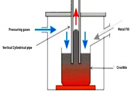
Our mathematical model equation was derived by considering a considering a vertical cylindrical pipe made of aluminum titanate immersed in molten aluminum (alloy
226) as shown in Figure 1. The pipe is immersed to a depth of 50mm. The total length of the pipe is 570mm and positive pressure relative to the air on the surface is applied which causes the melt in the pipe to rise to some height h.
Governing Equations
The mathematical model was derived by considering the total force acting on the liquid column (the kinetic energy and potential energy) and analyzing the causes of dissipation (friction due to the pipe wall and singular pressure loss at the entry) in the system. To get the total potential energy, the force acting in the liquid column is considered and integrated. Thus, the potential energy is given as:
$$ E _ {p} = \frac {1}{2} \rho g A h ^ {2} \tag {1} $$
The kinetic energy is given as:
$$ E _ {k} = \frac {1}{2} m v ^ {2} = \frac {1}{2} \rho A (h + H) \dot {h} ^ {2} \tag {2} $$ The total sum of energy in the column is obtained by summing up equations 1 and 2. The differentiated energy together with the 1st principle of thermodynamics gives the balance of energy equation. Energy lost due to dissipation is analyzed and incorporated into the sum of equations 1 and 2. The losses in the pipe are due to friction on account of the roughness of the wall and also due the singular pressure loss at the entrance or exit of the pipe if liquid rises or if liquid goes down respectively.
The energy loss due to friction can be written as:
$$ d E _ {w} = \frac {1}{2} k _ {w} \rho A \left(\frac {h}{H} + 1\right) \dot {h} ^ {2} | \dot {h} | \tag {3} $$ The singular pressure loss is given as:
$$ d E _ {E} = \frac {1}{2} k _ {E} \rho \dot {h} ^ {2} \left| \dot {h} \right| \tag {4} $$ Equations 5 and 6 are included in the sum of the potential and kinetic energy equation to obtain the total final equation:
( ) ( ) 2 ¨ 1 1 2 2 E w p t h h h H h gh k k h h H ρ (5) $$ \left(\left(h + H\right) \dot {h} + \frac {\dot {h} ^ {2}}{2} + g h\right) + \frac {1}{2} \left(k _ {E} + k _ {w} \left(\frac {h}{H} + 1\right)\right) \dot {h} | \dot {h} | = $$ where h is the height to which the liquid rises, and H is the length of pipe submerged under the liquid surface, E k is the coefficient of pressure lost at the entry of the pipe and KW the major coeffiecient of pressure lost is given by $$ K _ {w} = \frac {\lambda H}{2 r} $$ . λ is the friction factor and it is calculated from Moody’s diagram for a pipe made of Aluminium titanate with relative pipe roughness of 2.5.
Experimental Set-Up
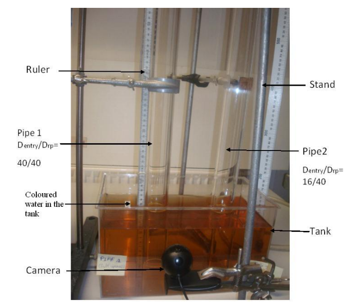
The experimental set-up (Figure 2) consists of a tank containing colored water. Two cylindrical pipes of the same pipe diameter but different entry diameters (Pipe 1: Diameter of entry/Diameter of rise pipe=40/40 and Pipe 2: Diameter of entry/Diameter of rise pipe=16/40) were immersed in a tank of colored water to the same depth. The initial height of the water in the tank is noted. A camera is attached to a laptop to record the experiment. Water is sucked to an initial height in Pipe 1 and then released. The same process is repeated for pipe 2. The initial height of water in the tank is noted.
Analysis of the Experimental Data
From the recordings, it was possible to determine the height of the first oscillation of pipe 1 and the frequency of both the pipes for the different initial conditions which is presented in summary form in Table 1. From Table 1, it is seen that pipe 2 is damped faster than pipe 1.
| Pipe 1: Dentry/Drp=40/40 | Pipe 2: Dentry/Drp=16/40 | ||||||
|---|---|---|---|---|---|---|---|
| Initial height of water in the tank (cm) | Initial height of water in pipe (cm) | Height of initial oscillation (cm) | Time taken for 10 oscillations (s) | Frequency (Hz) | Height of initial oscillation (cm) | Time taken for 10 oscillations (s) | Frequency (Hz) |
| 10 | 20 | 4.7 | 5.33 | 1.88 | 0.2 | 6.64 | 1.51 |
| 10 | 30 | 5.5 | 5.37 | 1.86 | 0.2 | 6.72 | 1.49 |
| 10 | 37 | 5.75 | 5.94 | 1.68 | 0.2 | 6.96 | 1.44 |
| 12 | 20 | 5.05 | 5.93 | 1.69 | 0.2 | 6.78 | 1.47 |
| 12 | 30 | 6.46 | 5.96 | 1.68 | 0.3 | 6.8 | 1.47 |
| 12 | 37 | 7.1 | 6.3 | 1.59 | 0.3 | N/A | N/A |
| 14 | 20 | 5.1 | 6.64 | 1.5 | 0.3 | 7.68 | 1.3 |
| 14 | 30 | 6.74 | 6.69 | 1.49 | 0.3 | 7.76 | 1.29 |
| 14 | 37 | 7.55 | 6.71 | 1.49 | 0.3 | 8.24 | 1.21 |
Table 1: From Table 1, it is seen that pipe 2 is damped faster than pipe 1.
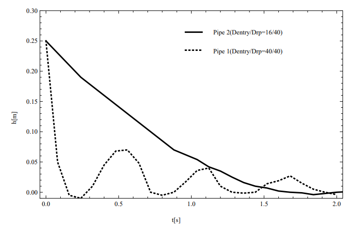
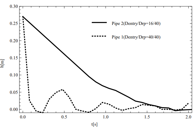
To compare the oscillations of the two pipes, the data of the oscillations is presented in the form of a graph. From the graphs presented in Figure 3 (initial height inside the pipes is 25cm) and Figure 4 (initial height inside the pipes is 27cm), it is clear that pipe 1 has higher oscillations than pipe 2. This is due to the fact that pipe 2 has a higher singular pressure loss at the entry due to the small diameter at the entry as compared to pipe 1.
Comparison of Experimental Results with Mathematical Model
To compare the experimental results with the mathematical model, different values of E K and W K had to be imposed in the mathematical model equation to closely follow the behavior of the experimental results. For the two pipes, the graph was plotted in Figure 4 and Figure 5.
![Figure 5: Graph of h[t] as a function of time for](/fulltextimages/9946/fig_5.png)
$$ r K _ {W} = 0. 0 9 3 7 5, K _ {E} = 0 a $$
and p = 0 and experimental data for pipe 1(Dentry/Drp
= 40/40) with an initial height of water in the pipe H0 = 25cm.
![Figure 6: Graph of h[t] as a function of time for](/fulltextimages/9946/fig_6.png)
$$ \mathrm {K} _ {\mathrm {W}} = 0. 0 9 3 7 5 \text {a n d} \mathrm {K} _ {\mathrm {E}} = 0. 5, $$
, p = 0 and experimental data for pipe 2(Dentry/
Drp = 16/40) with an initial height of water in the pipe H0 = 25cm.
It is noted that there is a big discrepancy between the mathematical model and the experimental results in terms of the height of initial oscillation and frequency. The experimental data shows lower height of initial oscillation for pipe 1 where the amplitude of the first oscillation is 0.06m as compared to the height of first oscillation of the mathematical model (0.2m). The frequency of the mathematical model is seen to be double that of the experimental data. For Pipe 2, the experimental data shows no oscillation but there is oscillation in mathematical model where the amplitude of the first oscillation 1.8cm.
To take care of the discrepancy, values of
E K were
imposed in the mathematical model. Different values were
investigated to check for which
E
K we would need to
impose to have approximately the same behavior as that of
the experimental results. The values imposed to obtain the
same behavior as in the experimental were
$$ K _ {E} = 1 4 \mathrm {(F i g u r e} $$
7 & Figure 8) for pipe 1(Dentry/Drp = 40/40) and
$$ \begin{array}{l} K _ {E} = 6 0 \\ (4 0) \mathrm {T h e} \\ \end{array} $$
(Figure 9 & Figure 10) for pipe 2(Dentry/Drp = 16/40). The W K
used for both pipes was
$$ K _ {W} = 0. 0 9 3 7 5. $$
![Figure 7: Graph of h[t] as a function of time for 0.09375 _W_ _K_ = , 14 _E_ _K_ = and p = 0 and experimental data for pipe 1(Dentry/ Drp = 40/40) with an initial height of water in the pipe H0 = 25cm.](/fulltextimages/9946/fig_7.png)
![Figure 8: Graph of h[t] as a function of time for](/fulltextimages/9946/fig_8.png)
$$ K _ {W} = 0. 0 9 3 7 5, K _ {E} = 1 4 $$
and p = 0 and experimental data for pipe 1(Dentry/Drp
= 40/40) with an initial height of water in the pipe H0 = 27cm.
![Figure 9: Graph of h[t] as a function of time for](/fulltextimages/9946/fig_9.png)
$$ K _ {W} = 0. 0 9 3 7 5, K _ {E} = 6 0 $$
and p = 0 and experimental data for pipe 2(Dentry/Drp
= 16/40) with an initial height of water in the pipe H0 = 25cm.
![Figure 10: Graph of h[t] as a function of time for](/fulltextimages/9946/fig_10.png)
$$ K _ {W} = 0. 0 9 3 7 5, K _ {E} = 6 0 a $$
and p = 0 and experimental data for pipe 2(Dentry/
Drp = 16/40) with an initial height of water in the pipe H0 = 27cm.
Conclusion
Experiments were done in order to visualize the behavior
of a column of water falling in a vertical pipe. It is seen that
for pipe 1 which has the same diameter at the entry as the
pipe diameter, there is a high oscillation of 4.5cm to 7.55 cm
depending on the initial conditions whereas for pipe 2 whose
entry diameter is not the same as the pipe diameter, the
oscillations are indistinguishable. The mathematical model
with the same initial conditions gives some results which are
close to the experimental data when imposed
14 E K = and 60 E K =
for pipe 1 and pipe 2 respectively. Using
$$ K _ {E} = 0 $$
(pipe 1) and
$$ K _ {E} = 0. 5 $$
(pipe 2), the Mathematical model
results are much different from the experimental results.
References
-
Boydak O, Savas M, Ekici B (2016) A numerical and experimental investigation of a high pressure die-casting Aluminium Alloy. International Journal of Metal Casting 10: 56-69.
-
Fu MW, Zheng JY (2022) Die Casting for Fabrication of Metallic Components and Structures. Encyclopedia of Materials: Metals and Alloys 4: 54-72.
-
Dalquist S, Gutowski T (2004) Life Cycle Analysis of Conventional Manufacturing Techniques: Sand Casting.
-
Cleary PW, Savage G, Ha J, Prakash M (2014) Flow analysis and validation of numerical modelling for a thin walled high pressure die casting using SPH. Computational Partical Mechanics 1: 229-243.
-
Fu J, Wang K (2014) Modelling and simulation of die casting process for a356 semi-solid alloy. Proceedia Engineering 81: 1565 -1570.
-
Davey K, Hinduja S (1990) Modelling the pressure die casting process with the boundary element: Steady state approximation. International Journal for Numerical Methods in Engineering 30(7): 1275-1299.
-
Kulasegaram S, Bonet J, Lewis RW, Profit M (2003) High pressure die casting simulation using a Lagrangian particle method. Communications in Numerical Methods in Engineering 19(9): 679-687.
-
Kurtulus K, Bolatturk A, Coskun A, Gürel B (2021) An experimental investigation of the cooling and heating performance of a gravity die casting mold with conformal cooling channels. Applied Thermal Engineering 194: 117105.
-
Dou K, Lordan E, Zhang Y, Jacot A, Fan Z (2021) A novel approach to optimize mechanical properties for aluminium alloy in High pressure die casting (HPDC) process combining experiment and modelling,” Journal of Materials Processing Technology 296: 117193.
-
Yazman S, Köklü U, Urtekin L, Morkavuk S, Gemi L (2020) Experimental study on the effects of cold chamber die casting parameters on high-speed drilling machinability of casted AZ91 alloy, Journal of Manufacturing Processes 57: 136-152.
-
Dørum C, Laukli HI, Hopperstad OS, Langseth M (2009) Structural behaviour of Al–Si die-castings: Experiments and numerical simulations. European Journal of Mechanics - A/Solids 28(1): 1-13.
- Sense, Gravity, Parity & Chirality in Mathematical Physics
- Quantum Lattice Simulations PHYSICS: Microcircuit Particle Formation and Observable Macroscopic Irreversible Time - A Discrete Lagrangian with Cellular Automata Framework
- Quantum Biology from Biomacromolecule to Cell, and Central Dogma Described by Quantum Theory
- Focus, Agility, Speed and Technology (FAST) for Sustainability and Growth
- Square Root Metric Geometry and Pati-Salam Model in Curved Space-Time
- A Simple System Demonstrating the Mpemba Effect in Classical Mechanics