Stability Analysis of Bread Wheat Genotypes Using the AMMI Stability Model at Southeast Oromia
Ethiopia is the largest wheat producer in Sub- Saharan Africa. The productivity of wheat has increased in the last few years in the country, but low as compared to other countries. This low productivity is attributed to a number of factors including biotic, abiotic, shortage of high yielding and stable varieties. The objective of the present study is to identify high yielding and stable genotype. A total of twenty genotypes including Dambal (st. check) and Mada walabu (Local check) were evaluated for two cropping season 2017 and 2018 at four locations: Sinana, Agarfa, Goba and Gololcha. The experiment was laid out in RCBD with three replications. The result of combined analysis of variance showed high significant differences for genotypes, environment and GE interaction. The result of AMMI analysis indicated that 36.3 %, of the total variability was justified by environment, 28.6% by genotypes and 34.9% by GE interaction whereas IPCA 1 and IPCA 2 explained 74.2% from the total GE. Based on GSI a single criteria for stability and high grain yield, genotypes G9, G1, G14,G10, G15 and G12 have the smallest genotype stability index which means they were stable and high yielding genotype. The best genotype with respect to environment Gololcha 2017 and Gololcha 2018 was genotype G10. Genotypes G3 and G17 were better adapted to environments Agarfa 2017. G12 is high yielder stable across tested locations. Therefore this genotype was identified as candidate genotypes to be verified for possible release.
Introduction
Ethiopia is leading wheat producer in Sub Saharan Africa and total production of 4.64 million tons CSA [1]. Accordingly, Oromia National Regional State contributes a total production of 2.67 million tons in the country. Among the wheat producing zones of Oromia, Arsi, West Arsi and Bale are considered as the wheat belts of eastern Africa. Although the productivity of wheat has increased in the last few years in the country, it is still very low as compared to other wheat producing countries in other parts of the world. The national average of wheat productivity is estimated to be 2.74 t ha-1 [1] (CSA, 2018), which is below the world average of 3.0 t ha-1 [2]. This low productivity is attributed to a number of factors including biotic, abiotic, shortage of high yielding and stable varieties.
In most of the plant breeding programs, GE interaction effects are of special interest for identifying the most stable genotypes, mega-environments and other adaptation targets. Various methods for yield stability analysis are based on different stability concepts and can be classified accordingly Flores, et al. Information regarding crop stability is applicable for selection of genotypes with constant yield across environments. Many of researchers have been reported to depict the responses of genotypes to the different condition of environments for simultaneous selection of yield and stability. These techniques are use statistical parameters to estimate stability of genotypes to variation in environments. Linear regression approach is used widely for identifying of high yielding and stable genotypes [3].
The additive main effect and multiplicative interaction (AMMI) method is an approach for evaluation of genotypes stability under different environments. The AMMI method merges principal components analysis and analysis of variance into an integrated approach and can be used to analysis of the multi-location experiments [4]. The AMMI analysis is effective because it provides agronomically meaningful interpretation of data [5]. The AMMI model is utilized for three main purposes [6, 7]. (i) to suitable in the initial statistical analyses of yield experiments, (ii) to summarize the relationships between genotypes and environments (GE) and (iii) to applicable for understanding complex genotypes × environment interaction effects. AMMI analysis has been applied extensively with great success to interpret genotype × environment interaction in wheat [8, 9]. A wider adapted Genotype performs consistently over a wider range of environment. The objective of this study was to select stable genotype and to identify promising genotypes.
Materials and Methods
Experimental Design and Methods
The experiment was conducted in four locations during 2017 and 2018 main cropping season at Sinana, Agarfa, Goba and Gololcha. The detailed description of environments given (Table 1). A total of twenty genotypes: including eighteen advanced genotypes, standard check Dambal and local check Mada walabu were tested using a randomized complete block design (RCBD) with three replications. A plot size of 6 rows with row spacing of 0.2 meter and row length of 2.5 meter was used and the four middle rows were used for data. Seed rate 150 kg ha-1 was used and drilling to the six rows. Fertilizer was applied 41 kg ha-1 N and 46 kg ha P2 O5 at planting.
| Location | Altitude (m) | Latitude | Longitude |
|---|---|---|---|
| Sinana | 2404 | 07 09.49’ | 40 13.77’ |
| Agarfa | 2486 | 07 15.29’ | 39 54.44’ |
| Goba | 2565 | 07 03.22’ | 39 59.04’ |
| Gololcha | 1970 | 07 45.04’ | 40 57.29’ |
Table 1: Experimental Area description.
Statistical Analysis
Mean grain yield data of the experiment were statistically treated by AMMI model analysis. This analysis consists in the sequential fitting of a model of analysis of experiments, initially by ANOVA (additive fitting of the main effects) and then by analysis of principal components (multiplicative fitting of the effects of interaction). The model AMMI equation is:
Yij=µ+gi+ej+∑n=1hλnαni.Ynj+Rij
Where ij Y is the yield of the ith genotype in the jth environment; µ is the grand mean; i g and je are the genotype and environment deviations from the grand mean, respectively; λn is the square root of the eigen value of the principal component Analysis (PCA) axis, αni and Ynj are the principal are the principal component scores for the PCA axis n of the ith genotype and jth environment, respectively and Rij is the residual. The analysis was done using GEA-R software (Genotype x Environment analysis with R for windows) version 4.1.
AMMI Stability Value (ASV)
The ASV is the distance from the coordinate point to the origin in a two dimensional of IPCA1 score against IPCA2 scores in the AMMI model [10]. Because of the IPCA1 score contributes more to the GE interaction sum of square, a weighted value is needed. This weight is calculated for each genotypes and environment according to the relative contribution of IPCA1 to IPCA2 to the interaction SS as follows: ASV= SSIPCA1/ SSIPCA2 (IPCA1score)2 + [IPCA2]2 Where, SSIPCA1/SSIPCA2 is the weight given to the IPCA1 value by dividing the IPCA1 sum squares by the IPCA2
sum of squares. The larger the IPCA score, either negative or positive, the more specifically adapted a genotype is to certain environments. Smaller IPCA score indicate a more stable genotype across environment.
Genotype Selection Index (GSI)
Based on the rank of mean grain yield of genotypes (RY) across environments and rank of AMMI Stability Value (RASV) a selection index GSI was calculated for each genotype which incorporate both mean grain yield and stability index in a single criterion (GSI) as suggested by Bose, et al. [11] and Bavandpori, et al. [12].
GSI = RASV + RY
Results And Discussions
Homogeneity of variance tests indicated homogenous error variance for grain yield in the eight environments allowed for a combined analysis across environments. The combined analysis of variance (Tables 2 & 3) indicated that the main effects of random environments and fix genotypes were significant for grain yield that exhibiting the presence of variability in genotypes and diversity of growing conditions at different environments. The combined analysis of variance was conducted to determine the effects of environment (location by year combination), genotype, and their interactions on grain yield of bread wheat genotypes (Table 3). The main effects of environment (E), genotypes (G) and GE interaction were highly significant at P < 0.01. Environment had the largest effect, explaining 74.6% of total variability, while genotypes and GE interaction explained 21.6 and 3.8% of total sum of squares, respectively (Table 3). A large contribution of the environment indicated that environments were diverse, with large difference among environmental means causing most of the variation in grain yield and higher differential in discriminating the performance of the genotype. The same result was reported by Farshadfar [13], Jacobsz, et al. [14] and Tadele, et al. [15]. Mean grain yield of genotypes was highest at Gololcha in 2018 cropping season, and at Sinana in 2017 cropping season. Similarly, mean grain yield of genotypes was lowest at Agarfa in 2018 (Table 2). Genotype G5 was the highest yielding at Goba 2017 and the lowest (Agarfa 2017) yielding environments. Genotypes G12, G19 and G10 showed 13.2, 4.7 and 1.2 tha-1 grain yield advantage over standard check (G5) respectively, and 86.1, 72.2 and 66.4 tha-1 grain yield advantage over local check (G11), respectively (Table 2).
| SN | Genotype Code | Year 2017 | Year 2018 | Mean | ||||||
|---|---|---|---|---|---|---|---|---|---|---|
| Sinana | Agarfa | Goba | Gololcha | Sinana | Agarfa | Goba | Gololcha | |||
| 1 | G1 | 4.2 | 3.4 | 5.6 | 4.7 | 3.6 | 3.1 | 4.3 | 4 | 4.11 |
| 2 | G2 | 4.4 | 3.5 | 5.1 | 4.2 | 3.3 | 3.1 | 3.5 | 4.4 | 3.95 |
| 3 | G3 | 3.6 | 3.9 | 4.6 | 3.6 | 3.7 | 3.6 | 4.4 | 3.9 | 3.91 |
| 4 | G4 | 4.3 | 3.4 | 4.6 | 4.7 | 3.6 | 3.3 | 3.4 | 5.1 | 4.05 |
| 5 | G5 | 5.2 | 3.5 | 5.8 | 4.2 | 3.3 | 3.5 | 3.4 | 5.2 | 4.26 |
| 6 | G6 | 4.3 | 4 | 4.7 | 3.4 | 3 | 3 | 3.5 | 5.1 | 3.89 |
| 7 | G7 | 4.2 | 4.2 | 3.8 | 4 | 2.6 | 3.4 | 3.6 | 4.8 | 3.85 |
| 8 | G8 | 4.7 | 3.9 | 4.9 | 3.5 | 2.7 | 3 | 3.2 | 4.4 | 3.78 |
| 9 | G9 | 4.7 | 4 | 4.3 | 3.9 | 2.3 | 3.7 | 4 | 5.1 | 4 |
| 10 | G10 | 4.4 | 5.2 | 4.9 | 4 | 3 | 3.5 | 4.6 | 5 | 4.31 |
| 11 | G11 | 2.8 | 0.8 | 1.8 | 4.8 | 2.1 | 1.4 | 1.8 | 5.2 | 2.59 |
| 12 | G12 | 5.5 | 5.5 | 5.4 | 4.4 | 3.6 | 3.7 | 5.1 | 5.3 | 4.82 |
| 13 | G13 | 5.3 | 3.6 | 4.2 | 3.5 | 3 | 2.9 | 3.1 | 4.7 | 3.78 |
| 14 | G14 | 3.9 | 3.9 | 3.9 | 3.8 | 2.9 | 2.7 | 3.4 | 4.4 | 3.61 |
| 15 | G15 | 4.7 | 4.8 | 4.3 | 3.9 | 3.5 | 2.9 | 3.8 | 4.5 | 4.06 |
| 16 | G16 | 4.1 | 3.2 | 3.9 | 3.9 | 2.7 | 2.6 | 4.4 | 4.3 | 3.63 |
| 17 | G17 | 4.2 | 4.6 | 4.1 | 3.7 | 3.7 | 2.9 | 4.6 | 4.2 | 3.99 |
| 18 | G18 | 2.6 | 2.6 | 1.9 | 3.8 | 2.8 | 2.2 | 3.5 | 4.1 | 2.97 |
| 19 | G19 | 5.3 | 4.9 | 5.3 | 3.7 | 3.9 | 3.6 | 4.5 | 4.4 | 4.46 |
| 20 | G20 | 4.4 | 3.8 | 3 | 3.8 | 3.3 | 2.2 | 3.8 | 4.2 | 3.63 |
Table 2: Mean performance of 20 bread wheat genotypes in 8 Environments.
| Source | d.f. | SS | MSS | SS% |
|---|---|---|---|---|
| Genotypes | 19 | 108.2 | 5.69** | 21.6 |
| Environments | 7 | 137.5 | 19.64** | 74.6 |
| Block | 16 | 14.6 | 0.914* | |
| Interactions | 133 | 132.7 | 0.998** | 3.8 |
| IPCA 1 | 25 | 61.8 | 2.47** | 49.2 |
| IPCA 2 | 23 | 31.4 | 1.37** | 25 |
| IPCA 3 | 21 | 19.8 | 0.94** | 15.8 |
| IPCA 4 | 19 | 12.5 | 0.66* | 10 |
| Residuals | 85 | 39.6 | 0.465 | |
| Total | 479 | 538.9 | 1.125 |
Table 3: ANOVA for grain yield of Bread wheat genotypes for the AMMI model.
AMMI model analysis: in AMMI model, principal component analysis is based on the matrix of deviation from additivity or residual will be analyzed. In this respect both the results of AMMI analysis, the genotypes and environment will be grouped based on their similar responses [5, 15, 16]. The result of AMMI analysis also showed that the first principal component axis (IPCA1) accounted for 49.2% over the interaction SS, IPCA2, IPCA 3 and IPCA4 explained 25.0%, 15.8% and 10.0% of the GE interaction SS, respectively. The first two IPCA scores were significant at (P<0.01%) and cumulatively accounted for 74.2% of the total GE interaction. This indicates that the use of AMMI model fit the data well and justifies the use of AMMI2.
d.f.=degree freedom, SS= Sum of square, MSS= Mean Sum of square, SS%= Percentage of sum of square, IPCA 1, 2, 3 and 4= first, second, third and fourth principal component AMMI Stability Value (ASV): ASV is the distance from zero in a two dimensional scattergram of IPCA1 scores against IPCA2 scores. Since the IPCA1 score contributes more to the GE sum of square, it has to be weighted by the proportional difference between IPCA1 and IPCA2 scores to compensate for the relative contribution of IPCA1 and IPCA2 total GE interaction sum squares. According to this stability parameter, a genotype with least ASV score is the most stable. The high interaction of genotypes with environments was also confirmed by high ASV and rank, suggesting unstable yield across environments. In general the importance of AMMI model is in reduction of noise even if principal components don’t cover much of the GE SS [5, 17].
Results of ASV parameter showed genotypes G9, G14, G7 and G16 as the most stable genotypes, respectively. The most unstable genotypes were G11 and G18 (Table 4). Although, ASV parameter was reported to produce a balanced measurement between the two first IPC’s (IPC1 and IPC2) scores, but it seems that this parameter is useful when the portion of explained total variation was relatively high [18].
Most of the time genotypes showed inconsistency in rank of grain yield across different tested environment; genotype ranked first in one environment may not be first at another tested environment. Hence, it is advantageous to look for a single criteria which help researchers to identify elite genotypes simultaneously for their high yielding and stable across tested environment. GSI (Genotype Selection Index) is a single criteria for stability and high grain yield which successfully used by Bose, et al. [11] and Bavandpori, et al. [12] to interpret interaction between genotype performance and environments. High yielding genotype with better stability has smallest values of GSI. The smallest Genotype Selection Index (GSI) exhibited by Genotypes G9 (GSI =9), G1 (GSI =11), G15 (GSI =14) and G10 (GSI =10). These genotypes were high yielder and comparatively stable. The Highest GSI (GSI=40) exhibited by genotype G11 which was highly unstable and lowest yielder among tested genotypes (Table 4).
| Genotype | Mean | ASV | RASV | RYI | GSI | CV% |
|---|---|---|---|---|---|---|
| G1 | 4.11 | 0.35 | 6 | 5 | 11 | 19.7 |
| G2 | 3.95 | 0.43 | 9 | 10 | 19 | 17.7 |
| G3 | 3.91 | 0.48 | 10 | 11 | 21 | 10 |
| G4 | 4.05 | 0.64 | 14 | 7 | 21 | 17.7 |
| G5 | 4.26 | 0.91 | 18 | 4 | 22 | 23.3 |
| G6 | 3.9 | 0.34 | 5 | 12 | 17 | 20.2 |
| G7 | 3.84 | 0.17 | 3 | 13 | 16 | 17 |
| G8 | 3.78 | 0.62 | 13 | 14 | 27 | 21.4 |
| G9 | 4.02 | 0.12 | 1 | 8 | 9 | 20.5 |
| G10 | 4.3 | 0.57 | 12 | 3 | 15 | 18.2 |
| G11 | 2.59 | 2.35 | 20 | 20 | 40 | 61.2 |
| G12 | 4.83 | 0.64 | 15 | 1 | 16 | 16.7 |
| G13 | 3.78 | 0.39 | 7 | 15 | 22 | 22.7 |
| G14 | 3.61 | 0.12 | 2 | 17 | 19 | 15.8 |
| G15 | 4.05 | 0.42 | 8 | 6 | 14 | 16.6 |
| G16 | 3.63 | 0.27 | 4 | 16 | 20 | 19.5 |
| G17 | 4 | 0.74 | 16 | 9 | 25 | 14.4 |
| G18 | 2.93 | 1.23 | 19 | 19 | 38 | 26.6 |
| G19 | 4.45 | 0.88 | 17 | 2 | 19 | 15.7 |
| G20 | 3.58 | 0.56 | 11 | 18 | 29 | 19.2 |
Table 4: Mean of 20 genotypes, AMMI stability values, Genotypic selection index and coefficient of variation. ASV= AMMI stability
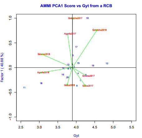
The vertex cultivars in each sector are considered best at environments whose markers fall into the respective sector. Environments within the same sector are assumed to share the same winner cultivars. Genotype-environment affinity depicted as orthogonal projections of the genotypes on the environmental vectors to identify the best cultivars with respect to environments. The best genotype with respect to environment Gololcha 2017 and Gololcha 2018 was genotype G10. Genotypes G3 and G17 were better adapted to environments Agarfa 2017 (Figure 1).
Conclusion
To develop varieties it is essential for breeders to evaluate their genotypes based on years and locations. Both yield and stability of performance should be considered simultaneously to reduce the effect of GE interaction and to make selection of genotypes more precise Based on ASV, genotype with least ASV scores are the stable and genotypes G9, G14, G7 and G16 were stable genotypes respectively. Based on GSI single criteria for stability and high grain yield genotypes G9, G1, G14, G10, G15 and G12 were found to be stable genotypes. G12 is high yielder stable across tested locations. Therefore this genotype was identified as candidate genotypes to be verified for possible release.
References
-
CSA (Central Statistical Authority) (2018) Agricultural sample survey 2017/18 Report on area and production of major crops for private peasant holdings, meher season. Statistical Central statistical agency Addis Ababa Ethiopia 584(1).
-
Hawkesford MJ, Araus J, Park R, Derini DC, et al. (2013) Prospects of doubling global wheat yields. Food and Energy Security (2): 34-48.
-
Alberts MJA (2004) A comparison of statistical methods to describe genotype × environment interaction and yield stability in multi-location maize trials. Plant Breeding MSc Thesis, University of the free state Bloemfontein, pp: 100.
-
Zobel RW, Wright MJ, Gauch HG (1988) Statistical analysis of a yield trial. Agron J 80: 388-393.
-
Gauch HG (1992) Statistical anlyis of regional yield trials. AMMI analysis of factorial designs 1st (Edn.), Elsevier, New York.
-
Gauch, HG (1988) Model selection and validation for yield trials with interaction. Biometrics 44: 705-715.
-
Crossa J, Gauch HG , Zobel RW (1990) Additive main effects and multiplicative interaction analysis of two international maize cultivar trials Crop Sci 30: 493-500
-
Petrovic S, Dimitrijevic M, Belic M, Banjac B, Boskovic J, et al. (2010) The variation of yield components in wheat (Triticum aestivum L) in response to stressful growing conditions of alkaline soil Genetika 4(3): 545-555.
-
Mohammadi M, Karimizadeh R, Hosseinipour T (2013) Parameters of AMMI model for yield stability analysis in durum wheat. Agric Con Sci 78: 119-124.
-
Purchase JL, Hatting H, Vandenventer CS (2000) Genotype x environment interaction of winter wheat in south Africa II. Stability analysis of yield performance. South Afr J Plant Soil 17: 101-107.
-
Bose LK, Jambhulkar N, Pande K, Sing O (2014) Use of AMMI and other stability statistics in the simultaneous selection of rice genotypes for yield and stability under direct-seeded conditions. Chilean Journal of Agriculture Research 74(1).
-
Bavandpori F, Ahmadi J, Hossaini SM, (2015) Yield Stability Analysis of Bread Wheat Lines Using AMMI Model. Agricultural Communications 3(1): 8-15.
-
Farshadfar E (2008) Incorporation of AMMI stability value and grain yield in a single non-parametric index (GSI) in bread wheat. Pak J Biol Sci 11(4): 1791-1796.
-
Jacobsz MJ, Merwe WJ, and Westhuizen MM (2015) Additive Main Effects and Multiplicative Interaction Analysis of European Linseed (Linum Ustatissimum L.) Cultivars under South African Conditions. Adv Plants Agric Res 2(3): 00049.
-
Tadesse T, Tekalign A, Sefera G, Mulugeta B (2017) AMMI Model for Yield Stability Analysis of Linseed Genotypes for the Highlands of Bale, Ethiopia. Plant 5(6): 93-98.
-
Gauch HG, Zobel Rw (1996) AMMI analysis of yield trials. In: Kang MS, Gauch HG (Eds.), Genotype by environment interaction. CRC press Boca Raton FL.
-
Pourdad SS, Mohammadi R (2008) Use of stability parameters for comparing safflower genotypes in multienvironment trials. Asian J Plant Sc 7: 100-110.
-
Sabaghnia N, Sabaghpour SH, Dehghani H (2008) The use of an AMMI model and its parameters to analyze yield stability in multi-environment trials. J Agric Sci 146: 571-581.
- The Role of Podocyte Apoptosis and the Involvement of SIRT1 in Diabetic Nephropathy
- Dealcoholization of Beer by Osmotic Distillation for the Beverage Industry
- Biopolymer-Based Edible Packaging- Biomaterials, Methods, and Applications in Food Industry: An Updated Review
- Influence of Bioprocessing Methods on 'China Rice' (Gawal R1), and Soyabean Supplementation on the Quality of Complementary Food
- Cassava (Manihot esculenta) Varietal Growth, Yield and Cyanide Content Performance in Three Sites in the South- Eastern Semi Arid Regions of Kenya
- Food Waste Treatment, Recycling, Management and Production of Value-Products-An Update on Methodologies and Current Trends