Assessment of Irrigation Potential in Jewuha Watershed, Middle Awash River Basin, Ethiopia
Ethiopia is endowed with immense water and land resources that could be tapped and used for irrigation development. However, little has been done so far due mainly to lack of comprehensive knowledge on the potential of these resources. This study was, therefore, taken up to assess the irrigation potential in data scarce Jewuha watershed of the Awash River Basin. To achieve the objective of the study, the suitability of the land for both surface and pressurized irrigations was estimated using a parametric evaluation technique combined with the FAO land evaluation framework in the GIS environment with multi-criteria analysis of irrigation suitability factors. The irrigation water demands of major crops adopted in the area were determined using CROPWAT software. The surface water potential at the sub watershed was estimated using a combination of SWAT model and the spatial proximity regionalization technique. The performance of the SWAT model was checked by statistical parameters. The irrigation suitability analysis reveals that 51372ha of the study area are suitable and 16274ha are unsuitable for surface irrigation system. Furthermore, 52768ha of the area are suitable and 15088ha are unsuitable for a sprinkler irrigation system. For drip irrigation, 52751ha are suitable and 14855ha are unsuitable. The calibration and validation of SWAT model showed that the model has performed well to simulate the hydrology of the watershed with a coefficient of determination (R2), Nash-Sutcliffe efficiency (NSE) and Percent of bias (PBIAS) of 0.74, 0.73 and 0.80 for calibration and 0.71, 0.70 and 7.90 for validation, respectively. From a combined analysis of the available land and water resources, the gross irrigation potential of the area is estimated to be 12,997ha, of which 3098ha of land is exclusively suitable for surface irrigation and 9,899ha is suitable for pressurized irrigation systems.
Introduction
Over 85 percent of Ethiopia’s population lives in rural areas and relies on agriculture for subsistence [1]. The
country has huge water resource potential that comprises 12 river basins with an annual runoff volume of 124 billion m3 of water and over 2.6 billion m3 of groundwater potential [2, 3]. But there is not sufficient water for most farmers to produce more than one crop per year due to a lack of water storage structures and large spatial and temporal variations in rainfall. Therefore, irrigation development and improved agricultural water management practices could provide opportunities to cope with the impact of climatic variability, enhance productivity per unit of land, and increase the annual crop production volume significantly [4].
Ethiopia also has a total cultivable land of between 30 to 70 million hectares out of 112 million hectares, but only 15 million hectares of land is under cultivation. However, only about 4% of this cultivated area has been irrigated so far [5], despite the fact that there is no precise figure for the potential and actual irrigated area. This is due to a lack of consistent, reliable inventory, well-studied and documented data. Also, this shows that there is a lack of detailed studies in the area. So, assessment of irrigation potential for irrigation development is important to utilize the land resources efficiently for the sustainable production of crops and to sustain the food security of the rapidly increasing population in the country [6]. Among the 12 river basins in Ethiopia, the Awash river basin is one of them, covering a total area of 110,000km2. The Awash river basin is the most intensively utilized river basin for irrigation development in Ethiopia due to its strategic location, accessibility, available land, and water resources [7]. However, the most utilized part is the upper part of the basin and relative to the total area, there is very little area to be utilized. Due to this, assessing irrigation potential in the Awash River basin is needed for more effective use of the basin for agricultural development.
Irrigation development could improve agricultural productivity and enhance socio-economic development through the growth of production [8]. But most of Ethiopia, particularly in the study area, practiced traditional agricultural activity. This shows that irrigation development in the study area is necessary and to do this, first the potential site for irrigation must be identified. Therefore, the objective of this study is to assess the irrigation potential for different irrigation systems in the Jewuha watershed to easily develop an irrigation project and the surface water resource potential.
The assessment of water availability at the watershed level is realized by quantifying runoff generated in the watershed. Water resources assessment relies on a full understanding of all the water flows and storages in the river basin or catchment under consideration has undertaken on many occasions in many countries of the world. The surface water potential in the Jewuha watershed was assessed using hydrological models. Some of the hydrological models for water assessment include unit hydrograph, empirical equation like rational method, IHACRES [9], SCS-CN [10], HBV [11], HEC HMS [12], WEAP [13], SWAT [14]. But unit hydrography and rational method is limited with area distribution that is useful only less than a catchment area of 500km2 and 50km2, respectively. SWAT performed better than IHACRES according to the statistical criteria [9]. Therefore, use of hydrological model for assessing the water resource in the watershed is more reliable and accurate due to this a physically based SWAT hydrological model is selecting for water resource assessment.
In the past, many studies have been done to assess surface water potential by using SWAT tool [15, 16, 17, 18, 19]. Furthermore, the irrigation water demand of the major crops adopted in the study area was estimated using the CROPWAT model [20].
Materials and Methods
Description of the Study Area
Jewuha watershed is located in the Awash River basin. It is geographically located between 39°44’55” to 40°10’4”E and 10°00’3” to 10°21’10”N. The watershed is 240km away from the capital city Addis Ababa in the northeast direction (Figure 1).
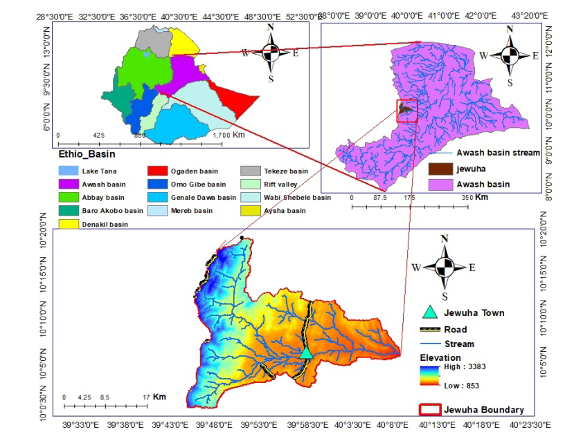
Figure 1: Location of the study area. The topography of the Jewuha watershed is characterized by diverse topographic conditions. The upper part of the watershed is characterized by mountainous and highly separated terrain with steep slopes and the downstream part is a gentle slope that is suitable for agricultural activity, with elevation ranges from 3555m in the mountainous area to 1101m in the lowland. The general topography of the catchments is undulating hills and flats.
The climate of the Jewuha watershed is characterized by high rainfall with low temperatures in the highland and low rainfall with high temperatures in the low land area. According to the Ethiopian agro-climatic zone classification, the climate of the study area ranges from hot temperate (Kola) around the low land of the Jewuha town area to cool temperature (wurch) in the mountains and escarpment.
Rainfall distribution over the area is bimodal, characterized by a short rainy season (Belg) that occurs between March and April and a long rainy season (kiremt) that occurs between June and August, with a dry season from December to February. In the dry season, the rainfall ranges between 218 and 259mm, whereas in the wet season it ranges between 600mm to 1500mm.
The temperature in the study area is hot in the low land areas, reaching up to 34.4℃ and the lowest temperature is recorded at Molale station on the highland, reaching up to 7℃ and sometimes it is less than this value.
The land use land cover map gives the spatial distribution and classification of the various land use land cover classes. Different land cover types have been found in the study area in terms of areal coverage. The important land cover units are forest, shrubs, grassland, intensively cultivated, woodland, bare areas, and built-up areas.
The types of soil found in the study area are Eutric Fluvisols, Vetric Cambisols, Leptosols, Eutric Cambisols, Chromic Cambisols, Chromic Vertisols, Haplic Xerosols, Eutric Regosols and Cambic Arenosols.
Data Types and Source
To achieve the objectives of the study, different data inputs were collected from various sources and field observations.
Meteorological Data
Meteorological data were collected from the National Meteorological Agency of Ethiopia (NMAE). Shewa Robit and Majeta climate stations were used for WGEN statistics calculation for SWAT using SWAT Weather database. The SWAT Weather Database Essenfelder [21] is designed to be a friendly tool to store and process daily weather data to be used with SWAT projects. It is capable of storing relevant daily weather information, easily generating.txt files that are used for input during SWAT project and efficiently calculating the WGEN statistics from one or more gauge stations. The daily weather data such as relative humidity (HMD), precipitation (PCP), solar radiation (SLR), maximum and minimum temperature (TMP), wind speed (WND) and the batch file containing the location of the gauge stations are loaded to SWAT Weather Database to calculate the WGEN statistics. The continuity and consistency of the meteorological data were checked by the normal ratio method and double mass curve, respectively.
Hydrological Data
The daily stream flow data of (1985-2003) at Jewuha, 1988-2001 at Ataye, and 1995 – 2011 at Robi gauging station were collected from the Ministry of Water, Irrigation and Energy (MoWIE). Ataye and Robi river were used for validation of the regionalization technique in model parameter transfer for the ungauged sub watershed.
Spatial Data
The data which is considered as spatial data includes DEM, land use land cover, soil map, and road map. Digital elevation model (DEM) was obtained from the USGS website. The soil chemical parameters of CaCO3 and EC covering the study area were obtained from the Harmonized World Soil Database (HWSD) on the FAO website, in Environmental System Research Institute (ESRI) shape file format and Micro Soft Access database Nachtergaele, et al. [22] and soil physical properties were obtained from the map of the Awash river master plan soil survey study from the GIS and remote sensing department in the Awash basin authority, Adama branch.
Land use land covers were obtained from the Water and Land Resource Center (WLRC), Addis Ababa; Ethiopia. The road map is another spatial data set that is used to extract road proximity to assess the irrigation potential of the study area and it is obtained from the DIVA-GIS website.
Land Suitability
Land suitability assessment means evaluating the parcel of land for irrigation or agricultural development [23]. Soil physical and chemical properties and topography, a characteristic of the land includes soil depth, texture, drainage, slope, CaCO3, EC and slope were taken to assess the suitability of the land in the study area. The digital soil map was prepared and obtained from different organizations, then analyzed in a GIS environment. The soil characteristics that were considered for land suitability assessment were taken from different works of literature [24, 25, 26, 27, 28].
Among the different land suitability assessment techniques, this study was interested in parametric evaluation systems prepared by Sys CE, et al. [25] based on the soil characteristics. Parametric procedures usually allocate numerical ratings to separate land characteristics or land qualities depending on their relevance to the land use considerations. Then, they are combined into one numerical result using a mathematical equation as shown Equation 1. These soil characteristics are rated and used to calculate the capability index (CI) (Table 1). The rating table was obtained from the tables prepared by [25].
- 100
- 100
- 100
- 100
- 100
- B
- C
- D
- E
- F
- CI
- A
- =
- ×
- ×
- ×
- ×
- × (1)
- Where CI is the Capability index for irrigation, A= soil texture rating, B = soil depth rating, C = CaCO3 rating, D = EC rating, E = drainage rating, F = slope rating
- Capability index Definition Symbol
- >80 Highly suitable S1
- 60 - 80 Moderately suitable S2
- 45 - 59 Marginally suitable S3
- 30 - 44 Currently not suitable N1
- <29 Permanently not suitable N2
Table 1: Capability indices (CI) class for land suitability.
SWAT Model Description
The water availability in the study area was assessed using the SWAT hydrological model. SWAT (Arnold JG, et al. [29] can simulate hydrological cycles, vegetation growth, and nutrient cycling with a daily time step by disaggregating a river basin into sub-basins and hydrologic response units (HRUs). SWAT uses the following water balance Equation 2 to simulate the hydrologic cycle within a watershed.
$$ S W _ {t} = S W _ {o} + \sum_ {i = 1} ^ {n} \left(R _ {d a y} - Q _ {s u r f} - E a - W _ {s e e p} - Q _ {g w}\right) $$ (2)
1 Where; SWt is the final water content (mm H2O), SWo is the initial soil water content on the day i (mm H2O), t is time, days, Rday is the amount of precipitation on the day i (mm H2O), Qsurf is the amount of surface runoff on the day i (mm H2O), Ea is the actual evapotranspiration on the day i (mm H2O), Wseep is the amount of water entering the vadose (unsaturated) zone from the soil profile on the day i (mm H2O), Qgw is the amount of return flow on the day i (mm H2O).
The model reflects the difference in evapotranspiration for various land use and soil type in the subdivision of watersheds. The runoff was predicted separated from each HRU and routed to obtain the total yield for the watershed. Hence, increase the accuracy and gives a better physical description of water balance.
Sensitivity Analysis
Sensitivity analysis is the way of determining the rate of change in model results concerning changes in model parameters [30]. Sensitivity analysis is important to provide information on the most important parameters that affect the process in the study area and helps to decrease the number of parameters in the calibration procedure by eliminating the parameters identified as not sensitive [31]. The sensitivity of the parameter was selected based on the P-test and t-test values. The value that has a high P and a low t value is the most sensitive parameter. The SUFI-2 (Sequential Uncertainty Fitting 2) program which is linked to SWAT-CUP Abbaspour C [30] was used for a combined model sensitivity and uncertainty analysis, calibration, and validation procedures. From the two sensitivity analysis techniques in SWAT-CUP; global sensitivity analysis technique was used.
Model Calibration and Validation
Calibration is an effort to better parameterize a model to a given set of local conditions, thereby reducing the prediction uncertainty [31]. The prediction of uncertainty of SWAT model calibration and validation results was analyzed by the SWAT calibration uncertainties program known as SWAT-CUP [30]. It is a public domain program that links Sequential Uncertainty Fitting (SUFI-2) [32], Particle Swarm Optimization (PSO) and Parameter Solution (ParaSol) Beven K, et al. [33] and Marko Chain Monte Carlo (MCMC). For this study, SUFI-2 was used for calibration of the model. To show the intimate relationship between the simulation result, expressed as 95PPU, and the observation expressed as a single signal (with some error associated with it), two statistics values are used [32]. These are the p-factor and r-factor, which give a good measure of the strength of calibration results. The P-factor is the percentage of measured data bracketed by the 95PPU band and the r-factor is a measure of the thickness of the 95PPU (Equation 3). The value of the p-factor and R-factor is between 0 and 1, and 0 to infinity, respectively. A p-factor of 1 and R-factor of 0 indicate simulations are exactly corresponding to the observed data [30].
( ) 1 ,97.5% ,2.5% n s s Q Q t t n t rfactor
$$ \cdot = \frac {\frac {1}{n} \sum_ {t = 1} ^ {n} \left(Q _ {t} ^ {s , 97.5 \%} - Q _ {t} ^ {s , 2.5 \%}\right)}{\sigma_ {o b s}} \tag {3} $$
1 obs σ Where ,97.5% s ti Q and ,2.5% s ti Q are the upper and lower boundary of the 95PPU at time t and simulation i, respectively, is the number of data points and is the standard deviation of the jth observed variable. Model validation is the process of describing that a given site-specific model is capable of making satisfactory simulations. It is the comparison of model results with an independent data set without further adjustment of the model parameters. Validation embraces running a model using parameters that were estimated during the calibration process and comparing the predictions to observed data not used in the calibration process. The hydrological data of Jewuha River from 1990 – 1997 and 1998 – 2003 was used for the calibration and validation of the SWAT model, respectively.
Model Performance Evaluation
Herein, the performance of the model was checked by statistical tests that can be used to judge the SWAT model. For this study, Nash Sutcliffe efficiency (NSE), percent bias (PBIAS), and coefficient of determination (R2) were used as recommended by Moriasi DNJG, et al. [34] (Table 2). The coefficient of determination (R2) describes the proportion of the variance in the measured data explained by the model (Equation 6). R2 ranges from 0 to 1, with higher values indicating less error variance, and typically, values greater than 0.5 are considered acceptable (Equation 4) [34].
Percent bias (PBIAS) (Equation 5) measures the average tendency of the simulated data to be higher or smaller than its observed values. The optimal value of PBIAS is 0.0, with lower magnitude values indicating an exact model simulation. The negative value of PBIAS indicates the models overestimate the simulated and the positive shows the model underestimates the simulated flow [34].
N
2 ( ) $$ T = 1 - \left| \frac {\sum_ {i = 1} ^ {N} \left(O _ {i} - 1\right)}{\sum_ {i = 1} ^ {N} \left(O _ {i} - 2\right)} \right| $$ i Pi Oi NSE ( )
2 1
1 (4) $$ \sum_ {i = 1} ^ {N} \left(O _ {i} - \bar {c}\right) $$
i Oi Oi
1 N
( )
1 100 i x Pi Oi PBIAS
$$ T = \left| \frac {\sum_ {i = 1} ^ {N} \left(O _ {i} - 1\right)}{\frac {N}{\sum}} \right| $$ (5) ∑ = i Oi
1
2 N
( )( )
$$ \sum_ {\mathrm {i} = 1} ^ {\mathrm {N}} \left(\mathrm {O} _ {\mathrm {i}} - \bar {\mathrm {O}}\right) \left(\mathrm {P} _ {\mathrm {i}} - \bar {\mathrm {P}}\right) $$
- $R^{2}=\left[\frac{i=1}{\sqrt{\sum_{i=1}^{N}\left(O_{i}-\bar{O}^{2}\right)\sqrt{\sum_{i=1}^{N}\left(P_{i}-\bar{P}\right)^{2}}}}\right]$
Table 3: General performance rating [34,36].
Where Pi = simulated flow, Oi = observed flow, i O = the mean of observed data, P ̅ is predicted flow and the remaining variable is stated above and N is the total number of observations.
The Nash–Sutcliffe efficiency (NSE) Sutcliffe JE, et al. [35] (Equation 4) indicating how well the model expresses the variance in the observation. It generally ranges from - ∞ to 1 the optimum value is unity and it shows a good explanation of the observed versus simulated data fits on a one to one line (Table 2).
| Performance rating | NS | PBIAS | R² |
|---|---|---|---|
| Very good | 0.75 < NS < 1 | PBIAS < ±10% | 0.75 < R² < 1 |
| Good | 0.65 < NS < 0.75 | ±10% < PBIAS < ±15% | 0.65 < R² < 0.75 |
| Satisfactory | 0.5 < NS < 0.65 | ±15% < PBIAS < ±25% | 0.5 < R² < 0.65 |
| Unsatisfactory | NS < 0.5 | PBIAS > ±25% | R² < 0.5 |
Table 2: General performance rating [34,36].
Regionalization Technique for Ungauged Sub Watershed
Regionalization is the process of transferring hydrological information (parameters) of a model from a gauged watershed to an ungauged watershed.
Among the different regionalization techniques, spatial proximity and physical similarity methods are widely used [37, 38]. In this study, spatial proximity with Inverse Distance Weighting (IDW) was used to transfer the calibrated model parameter of the gauged watershed to the ungauged watershed. And IDW was used to estimate the weight of the ungauged watershed. The distance between the two watersheds was determined using GIS. This regionalization techniques were verified using leave-one-out cross validation, in which a single gauged site is considered as ungauged and the transferred parameters to that site are entered into the SWAT-CUP to validate with the observed flow. Observed flow at Jewuha and the two neighboring watersheds of Shewa Robit and Ataye gauged watersheds was used to estimate the flow in the ungauged sub-watershed of the Jewuha River. The calibrated parameters of the Jewuha and Robi watersheds were transferred to the other ungauged sub watersheds. The parameters transferred by this technique are added into the SWAT model using a manual calibration helper and then the SWAT model is run to obtain the flow for each sub watershed. The general formula for spatial proximity with the IDW method to regionalize the calibrated parameter of the gauged watershed is as follows (Equations 7 and 8).
ug n w Z zi i i = ∑ =
(7)
1
Where is the estimated model parameter at the ungauged watershed; n is the total number of observed points (gauges); is the calibrated parameter value at gauged watershed and is the weight contributing to the interpolation
Where is the distance between at the centroids of gauged and ungauged watershed .
Estimation of Irrigation Water Demand
Irrigation water demand is estimated from the water requirement of the crop. The major crops adopted in the study area include maize, cabbage and onion. Several methods and procedures are available to compute the crop water requirement. The computer program available in FAO Irrigation and Drainage Paper No. 56 “CROPWAT” has been used for the calculation of crop water requirements (Equation 9).
$$ E T _ {c} = K _ {c} \times E T _ {o} \tag {9} $$
Where Kc is crop coefficients and ETc is crop evapotranspiration in mm.
Irrigation water demand is derived from crop evapotranspiration (ETc) and effective rain fall which is calculated based on USDA soil conservation service. Then the net irrigation water demand of the crop was calculated as follows (Equation 10).
$$ N I W D = E T _ {C} - P _ {e f f} \tag {10} $$
The gross irrigation water demand of the crop has been calculated by considering the loss of water during application of water to the irrigation field, loss in the canal through seepage and evaporation (Equation 11). Thus, so as to compensate for this loss, irrigation efficiency was introduced. The irrigation project efficiency is between 0.45 and 0.7 for surface irrigation and 0.7 to 0.9 for pressurized irrigation systems [39]. Thus, for this study, average irrigation efficiency was taken as 0.5, 0.75 and 0.85 for surface, sprinkler and pressurized irrigation systems, respectively.
NIWD GIWD η = (11)
Irrigation Suitability Area Assessment
The irrigation suitability of the study was assessed by weighing the factors of land suitability, land use land cover, distance from the source, and distance from the road [40, 41, 42].
Land Use Land Cover Suitability Assessment
The LULC of the study were reclassified based on the classification system of (FAO, 1976) using the reclassification tool, which is an attribute generalization technique in ArcGIS, as highly suitable (S1), moderately suitable (S2), slightly suitable (S3) and not suitable (N) (Table 3).
| LULC type | Definition | LULC rating (r) | Class | |
|---|---|---|---|---|
| Cultivated land | Highly suitable | 4 | S1 | |
| Grassland/bare land | Moderately suitable | 3 | S2 | |
| Shrub/bush/wood land | Slightly suitable | 2 | S3 | |
| Settlement/forest/wetland | Not suitable | 1 | N |
Table 4: Land use land cover suitability rating [41,43]. Distance from the Water Source (River) Suitability Assessment The identi
Table 3: Land use land cover suitability rating [41, 43]. Distance from the Water Source (River) Suitability Assessment The identification of irrigable land that is close to the water supply (rivers) was done by calculating the straight- line (Euclidean) distance from the streams that is generated from a 20m x 20m cell size DEM in a GIS tool and then reclassifying. The land which is nearest to the stream was considered the most suitable land for irrigation development and the land which is far from the stream is slightly suitable [26, 44]. The land from the river was reclassified as highly suitable (S1), moderately suitable (S2), slightly suitable (S3) and not suitable (N) (Table 4).
| Class | Definition | Rating (r) | Distance from river (Km) | |
|---|---|---|---|---|
| S1 | Highly suitable | 4 | 0 – 2 | |
| S2 | Moderately suitable | 3 | 2 – 4 | |
| S3 | Slightly suitable | 2 | 4 – 5 | |
| N | Not suitable | 1 | >5 | |
| Factor | Soil | LULC | Distance from river | Distance from road |
| Soil | 1 | 2 | 3 | 4 |
| LULC | 1/2 | 1 | 2 | 3 |
| Distance from river | 0.333 | 0.5 | 1 | 2 |
| Distance from road | 0.25 | 0.333 | 0.5 | 1 |
| Sum | 2.08 | 3.833 | 6.5 | 10 |
Table 5: Distance from source suitability rating [27,44].
Distance from Road Suitability Assessment
The road map obtained from the DIVA-GIS website were reclassified based on the classification system of FAO [23] using the reclassification tool in the GIS. It is classified as highly suitable (S1), moderately suitable (S2), slightly suitable (S3) and not suitable (N) by ratings of 4, 3, 2, and 1, respectively (Table 5).
| Class | Definition | Rating (r) | Distance from road (Km) |
|---|---|---|---|
| S1 | Highly suitable | 4 | 0-3 |
| S2 | Moderately suitable | 3 | 3-5 |
| S3 | Slightly suitable | 2 | 5-8 |
| N | Not suitable | 1 | >8 |
Table 6: Distance from road suitability rating [26].
Weighted Overlay of Irrigation Suitability Factors
To find an overall suitable site for irrigation, a suitability model was created using the model builder in the GIS Arc tools box to overlay the factor to map the suitable land. The weights developed above for each factor were overlaid in GIS to undertake multi-criteria evaluation (MCE) [45]. In a multi- criteria evaluation, an attempt is made to combine a set of criteria to achieve a single composite basis for a decision according to a specific objective. The relative importance/ weight of criteria and sub-criteria was estimated using multi- criteria evaluation through AHP, applied by using pairwise comparison of each suitability factor developed by Saaty L [46].
In pairwise comparison, each factor was matched head-to-head (one to one) with the other and a pairwise or comparison matrix was prepared to express the relative importance. The diagonal elements of the pairwise comparison matrix are assigned the value of unity since the diagonal of the matrix value was obtained by the compared value of itself (Table 6).
To fill the matrix, ratings were given for all factors on a 9 point continuous scale. For example, if one feels that land suitability is very strongly more important than LULC suitability in determining whether it is suitable for irrigation, one will enter 7 on this scale. However, if the reverse is true, one will give the value of 1/7. The value is given based on expert judgment and related literature reviews.
$$ N = \frac {\sum j}{c} $$
(12) Where N is normalized value, j is the column of the matrix and c is the values of the column of the factors
| Soil | LULC | Distance from river | Distance from road | |
|---|---|---|---|---|
| Land | 0.48 | 0.52 | 0.46 | 0.4 |
| LULC | 0.24 | 0.26 | 0.31 | 0.3 |
| Distance from river | 0.16 | 0.13 | 0.15 | 0.2 |
| Distance from road | 0.12 | 0.09 | 0.08 | 0.1 |
Table 7: Normalized value of factors The Eigenvectors and weights of the criteria were calculated from the normalized matrix thro
| Eigenvectors | |
|---|---|
| Land | 1.86 |
| LULC | 1.11 |
| Distance from river | 0.64 |
| Distance from road | 0.39 |
Table 8: Eigenvector value of criteria
$$ W _ {i} = \frac {\sum N}{x} \tag {13} $$
x Where the weights of the criteria, N is the row values of normalized matrix and x is the number of criteria for suitability analysis.
With a weighted linear combination, factors are combined by applying weight or percent of influence to the suitability of the irrigation obtained by the pairwise comparison technique. The multiplication was based on the following Equation 14.
X i n $$ S _ {i} = \sum_ {i = 1} ^ {n} W _ {i} $$
(14) Where S suitability, Wi is the weight of factor, Xi is criteria score of factor available water in the river in volume.
The map obtained after overlaying was irrigation suitability, which are classified based on their degree of suitability as highly suitable (S1), moderately suitable (S2), slightly suitable (S3) and not suitable (N) (FAO 1976) (Table 9).
| Class | Definition | |
|---|---|---|
| 4 | S1 | Highly suitable |
| 3 | S2 | Moderately suitable |
| 2 | S3 | Slightly suitable |
| 1 | N | Not suitable |
Table 9: Irrigation suitability rating
Irrigation Potential Area Assessment
Irrigation potential (IP) is the land that is suitable for irrigation and that can be irrigated with the available surface water at a selected diversion site.
Diversion sites are selected by considering different factors. Those includes, diversion site elevation must be larger than the area being irrigated, it should be easily accessed by road, the site should be not be too far from the command area of the project Dai X [47] and the river cross section should be straight and narrow.
After the estimation of suitable land, irrigation water demand and available surface water, the actual irrigation potential of the study area was estimated. The actual irrigation potential at the selected diversion site was evaluated using Equation 15 for each perennial and some intermittent rivers in the watershed.
$$ I P (h a) = \frac {A W}{G I W D} \tag {15} $$
Where GIWD (m3/ha) is gross irrigation water demand and AW (m3) is available water in the river at selected diversion site in m3/ha or mm (1mm = 10m3/ha) The irrigation potential areas which are estimated for each diversion site might not be found along the river and its delineation is difficult. In such case, manual delineation through trial and error was done by following the contour line generated.
Result and Discussion
Land Suitability for Irrigation Potential
The primary purpose of irrigation land suitability classification is to establish the extent and degree of suitability (arability) of lands for sustained irrigation farming to serve as a basis for selecting lands to be included in irrigation agriculture.
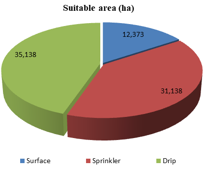
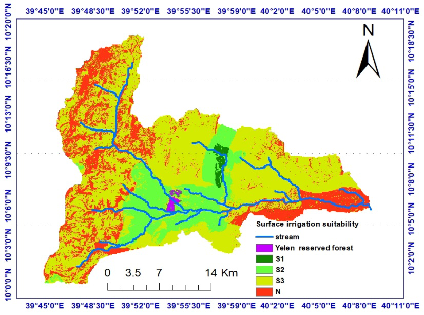
In this study, it has been analyze and compare the surface and two pressured (i.e. sprinkler and drip) irrigation methods by considering five soil characteristics and slope of the topography based on the parametric evaluation system as described by Sys CE, et al. [25]. The result showed that about 12,373ha of land are range in between moderately to marginally suitable for surface irrigation, 31,138ha of land are range in between highly to marginally suitable for sprinkler irrigation system and 35,433ha of land are considered highly to marginally suitable for drip irrigation systems (Figure 2). The value of land capability indices (CI) in the study area ranges from 17 to 70 for surface irrigation, 18 to 81 for sprinkler irrigation and 23 to 86 for drip irrigation.
When comparing the land suitability for the three irrigation systems in the study area 23,060ha of land is more suitable for drip irrigation than surface irrigation and 4295ha of land are additionally suitable for drip irrigation than sprinkler irrigation and 18,765 area of land are more suitable for sprinkler irrigation than surface irrigation systems. Generally, the land of the study area is more suitable for pressurized irrigation system (sprinkler and drip) than surface irrigation system due its high area coverage of steep slope greater than 8% in the watershed that are not suitable for surface irrigation systems. This result is similar with the work of Albaji M, et al. [24] Comparison of different irrigation methods based on the parametric evaluation approach in North Molasami plain, Iran.
Land Use Land Cover Suitability
Different land use land covers in the study area were identified and give a suitability rating factor based on their importance for irrigation development costs to remove or change for cultivation and environmental impacts under the watershed. After rating factor was given for the land use types, reclassified map of the study area was developed as shown below in Figure 3. The land use type was reclassified based on the FAO [23] land suitability classification systems, the land use type was reclassified as 31,492ha highly suitable (S1) which is Cultivable land, 5756ha moderately suitable (S2) which is grass land/bare land, 30,599ha marginally/ slightly suitable (S3) which is shrub/bush/wood land), and 105ha not suitable (N) which include settlement/forest/wet land. The similar study which is conducted by Rediet, et al. [41] land suitability evaluation for surface irrigation using spatial information technology in Omo Gibe basin, Ethiopia reclassified the land use as similar with this study. And also, Gurara [43] Evaluation of Land Suitability for Irrigation Development and Sustainable Land Management Using ArcGIS on Katar Watershed in Rift Valley Basin reclassified the land with a similar fashion.
![Figure 3: The land use type was reclassified based on the FAO [23] land suitability classification systems, the land use type was reclassified as 31,492ha highly suitable (S1) which is Cultivable land, 5756ha moderately suitable (S2) which is grass land/bare land, 30,599ha marginally/ slightly suitable (S3) which is shrub/bush/wood land), and 105ha not suitable (N) which include settlement/forest/wet land. The similar study which is conducted by Rediet, et al. [41] land suitability evaluation for surface irrigation using spatial information technology in Omo Gibe basin, Ethiopia reclassified the land use as similar with this study. And also, Gurara [43] Evaluation of Land Suitability for Irrigation Development and Sustainable Land Management Using ArcGIS on Katar Watershed in Rift Valley Basin reclassified the land with a similar fashion.](/fulltextimages/12277/fig_3.png)
Distance from River and Road Suitability
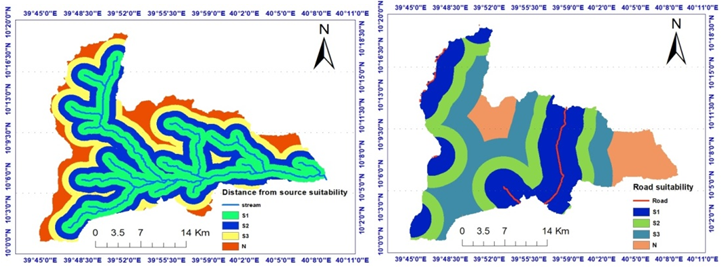
It is important to make sure that there were no lacks of irrigation water supply due to the problem of far distance to the river. If water is in short supply during some part of the irrigation season, crop production was suffering, returns are decline and parts of the scheme’s investment are laid idle. Also when the irrigation potential area is very far from the stream it needs construction of long canal thus this increase the cost of construction and the development of irrigation project is not feasible.
Thus, the result of the analysis to estimate the suitability of the land from stream revealed that 27,991ha of land are highly suitable, 18,780ha are moderately suitable 12,412ha of land are slightly suitable and 8779ha are not suitable for irrigation development.
As shown in the map (Figure 4), most of the area is highly suitable from road accessibility which means the irrigable area is near to a major road to transport the products to market area and again farm machineries to the farm land. The result of road suitability shows that 21,620ha of land are highly suitable, 17,256ha are moderately suitable, 18,257ha are slightly suitable and 10,830ha are not suitable for irrigation. The similar study by Worqlul, et al. [26] and Nigussie, et al. [40] the land which is nearest to the stream and road was considered as the suitable land for irrigation development and the land which are far from the stream are slightly suitable.
Surface Water Potential
Surface water of the study area was assessed using SWAT hydrological model. The model in the study area can be performed well with good performance.
SWAT Model Sensitivity Analysis
Among twenty one model parameters that were selected for sensitivity analysis, sixteen parameters were found to be sensitive under the category from high to low sensitive.
The most sensitive parameters of the study area in the SWAT model are R_CN2, ALPHA_BF, R_ESCO, R_EPCO, V_GW_ DELAY, V_ALPHA_BF, V_GWQMN, V_GW_REVAP, V_REVAPMN, V_RCHRG_DP, R_SOL_AWC, R_SOL_K, R_SLSUBBSN, R_ SURLAG, R_HRU_SLP, V_SHALLIST.gw and R_OV_N. Among these sensitive model parameters, curve number (R_CN2), saturated hydraulic conductivity (R_SOL_K), Ground water delay (days) (V_GW_DELAY), Manning’s “n” values for overland flow (R_OV_N) and available water capacity of the soil layer (R_SOL_AWC) are the top five sensitive parameters with a p-value less than 0.5.
Model Calibration and Validation
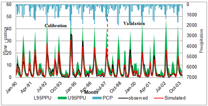
Using the river discharge data obtained from the Minister of Water, Irrigation and Energy (MoWIE), the SWAT model was calibrated at a monthly time scale (Figure 5).
Model Performance Evaluation
The performance of the model was evaluated using time series plots of observed and simulated value and statistical measures such as coefficient of determination (R2), Nash- Sutcliffe efficiency (NSE) and percent of bias (PBIAS). The statistical analysis of the watershed showed very good agreement between observed and simulated monthly flow. For the Jewuha watershed, the model overestimates the flow. The model was most affected by small traditional diversion structures in the Jewuha watershed, which do not have sufficient data to enter the value into the SWAT model. This makes the model perform less. The p-factor is a good measure of the strength of calibration results. The P-factor is the percentage of measured data bracketed by the 95PPU band and its value is range between 0 and 1. When its value ranges between 0.7 and 1 the percentage of uncertainty is very good. As shown in Table 10, the p-factor was 0.75 for the Jewuha River. This value shows that the 95PPU band is within acceptable ranges in the watershed. Inline with this study by Beza Manamno, et al. [48] for modeling and assessing surface water potential using SWAT model spatial proximity regionalization technique, the performance of the model was very good with a statistical indices greater than 0.7.
| Objective function | Calibration | Validation |
|---|---|---|
| R2 (Coefficient of determination) | 0.74 | 0.71 |
| NSE (Nash Sutcliff Efficiency) | 0.73 | 0.7 |
| PBIAS (Percent of bias) | -0.8 | 7.9 |
| RSR | 0.51 | 0.54 |
| p-factor | 0.75 | 0.74 |
Table 10: Model performance
Flow Regionalization
The flow from the gauged watershed to the ungauged watershed was estimated through parameter regionalization using the spatial proximity (SP) technique by Inverse Distance Weighting (IDW). For verification of the regionalization technique in the watershed, the statistical parameters of the objective function are good and this shows that applying the spatial proximity technique to transfer the model parameters to ungauged sub watershed to estimate was acceptable. Thus, the flow in the ungauged sub watershed was estimated using the spatial proximity (SP) regionalization technique and shown in the Table 11 below.
| Sub Watershed | Jan | Feb | Mar | Apr | May | Jun | Jul | Aug | Sep | Oct | Nov | Dec |
|---|---|---|---|---|---|---|---|---|---|---|---|---|
| Gida | 0.5 | 0.97 | 0.87 | 0.83 | 0.8 | 0.4 | 1.06 | 2.62 | 1.83 | 1.13 | 0.8 | 0.7 |
| Lomi | 4.1 | 4.62 | 5.75 | 6.92 | 4.1 | 1.8 | 8 | 21.5 | 14.54 | 8.14 | 5.22 | 4.3 |
| Gundifit | 1.1 | 2.13 | 2.52 | 3.54 | 2.7 | 1.6 | 5.43 | 8.29 | 6.24 | 3.61 | 2.4 | 1.6 |
| Ashmaq | 0.1 | 0.42 | 0.5 | 0.74 | 0.5 | 0.3 | 1.24 | 1.77 | 1.09 | 0.46 | 0.3 | 0.2 |
| Samet | 0.4 | 0.78 | 0.9 | 1.3 | 0.9 | 0.6 | 2.35 | 2.99 | 1.77 | 0.9 | 0.7 | 0.5 |
Table 11: Mean monthly stream flow (m3/s) of ungauged sub watershed using spatial proximity regionalization.
Irrigation Water Demand
CROPWAT model results include crop evapotranspiration (ETc) and effective rainfall to estimate the irrigation water requirement of the crop. As shown in Table 12, monthly gross irrigation water requirement of maize, cabbage and onion was estimated throughout their full growth periods for both surface, sprinkler and drip irrigation systems.
| Crop type | Jan | Feb | Mar | Apr | May | |
|---|---|---|---|---|---|---|
| Surface irrigation | Onion | 135.15 | 59.3 | 89.85 | 37 | 0 |
| Surface irrigation | Maize | 69.36 | 50.66 | 120.57 | 144 | 119.94 |
| Surface irrigation | Cabbage | 123.74 | 83.41 | 144.21 | 74.6 | 0 |
| Surface irrigation | Average | 109.42 | 64.46 | 118.21 | 85.2 | 39.78 |
| Sprinkler irrigation | Onion | 90.1 | 39.53 | 59.9 | 24.7 | 0 |
| Sprinkler irrigation | Maize | 46.24 | 33.77 | 80.38 | 96 | 79.96 |
| Sprinkler irrigation | Cabbage | 82.5 | 55.6 | 96.1 | 49.7 | 0 |
| Sprinkler irrigation | Average | 72.95 | 42.97 | 78.79 | 56.8 | 26.65 |
| Drip irrigation | Onion | 79.5 | 34.88 | 52.85 | 21.8 | 0 |
| Drip irrigation | Maize | 40.8 | 29.8 | 70.92 | 84.71 | 70.55 |
| Drip irrigation | Cabbage | 72.8 | 49.1 | 84.8 | 43.9 | 0 |
| Drip irrigation | Average | 64.37 | 37.93 | 69.52 | 50.14 | 23.52 |
Table 12: Gross irrigation water demand (mm/month).
Irrigation Suitability Potential
To find the irrigation suitability potential of the study area; land suitability maps, land use land cover suitability maps, distance from stream suitability maps and distance from road suitability maps were overlay in a GIS environment using a weighted overlay analysis tool in the spatial analysis tool. A similar work studied by Worqlul, et al. [26] in the lake Tana basin of Ethiopia considers all these factors to assesses the irrigation potential for surface irrigation but it does not assess the area for pressurized irrigation systems. To overlay these maps, the factors are given a weight. Based on the pairwise comparison of the factors, land suitability was given a highest weight and distance from road suitability was given the list weight (Table 13). Similarly a study which is conducted in the Blue Nile Basin by Nigussie, et al. [40] gives the highest weight for soil/land characteristics, but they are not consider road/market proximity.
| Wj (Weight (%) | |
|---|---|
| Land suitability | 47 |
| Land use land cover suitability | 27 |
| Distance from source suitability | 16 |
| Distance from road suitability | 10 |
| Sum | 100 |
Table 13: Weight developed for factors.
The consistency ratio (CR) was 0.02, which is acceptable for weighting the factors to evaluate the irrigation suitability of the watershed. Surface Irrigation Suitability The distinction in land suitability for surface and pressurized (Sprinkler and Drip) is basically made based on land slope. Surface irrigation is considered suitable for land slopes less than 8% due to difficulties in water control and distribution on steeper land slopes.
Sprinkler Irrigation Suitability
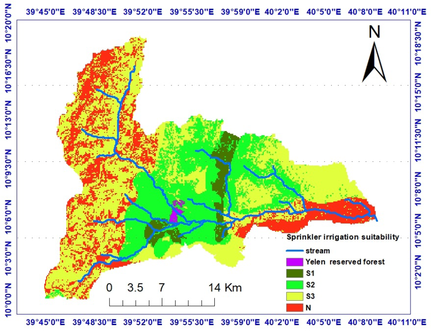
From the total land area of the study 67,274ha, 52768ha of land can be developed by the sprinkler irrigation system which means they are suitable for sprinkler irrigation systems and 23% (15088ha) are not suitable to develop a sprinkler irrigation system. Of the total suitable land from the study area 4.5% (3029ha) are highly suitable, 26.5% (18042ha) are moderately suitable, and 46% (31697ha) are slightly suitable for sprinkler irrigation systems (Figure 7). The analysis indicates that high portion suitable area can be observed in the largest part of the cultivated area, located in the middle part of the study area due to deep soil, good drainage, texture, salinity and slope in between 8% to 15%. AS seen from the map (Figure 7), the unsuitable area is located in the west and highland area due to its rugged topography and low soil depth, less than 30cm depth.
Drip Irrigation Suitability
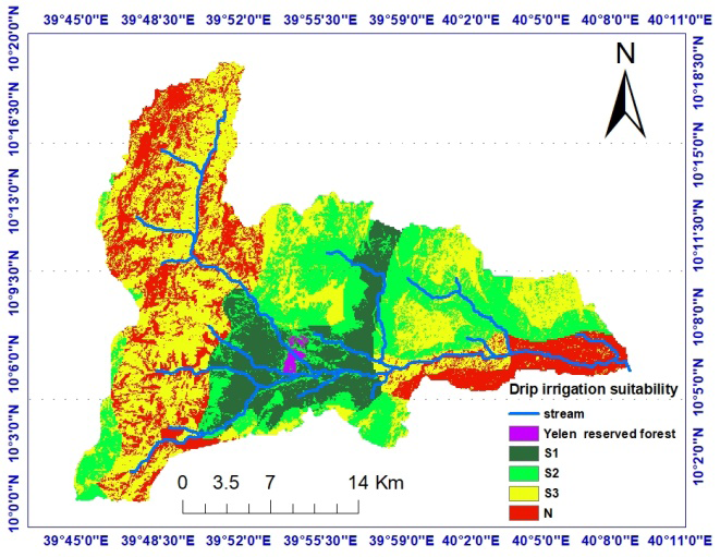
The assessment of drip irrigation suitability in the study area revealed that 13% (8498ha) are highly suitable, 25% (16971ha) are suitable, 40% (27282ha) are moderately suitable, and 22% (14855ha) are not suitable for drip irrigation system. From the total land area of the study, 52751ha of land can be developed by the drip irrigation system (Figure 8). Due to its suitability for any type of topography up to 30% slope and also avoids water loss more than surface irrigation methods the study area is more suitable for drip irrigation systems. Pressurized (sprinkler and drip) irrigation systems can increase food production and water conservation in developing countries like Ethiopia where the need is high however; it is affected by water quality.
Herein, the comparison of the different types of irrigation revealed that drip irrigation was more effective and efficient than the sprinkler and surface irrigation methods and improved land suitability for irrigation purposes. The second best option was the application of sprinkler irrigation which was considered as being more practical than the surface irrigation method. The main limiting factor for both irrigation system was high slope and low soil depth in the study area.
Irrigation Suitability of River Catchments (Sub Watershed)
The irrigation suitability of river catchments or sub watersheds as shown in Table 14 below shows that 315ha of the area in Gida sub watersheds was categorized as highly suitable for surface irrigation, but the remaining sub watersheds are not considered as highly suitable. For sprinkler irrigation suitability system 587ha, 603ha and 2ha of the area in Gida, Gundifit and Ashemaq are categorized under highly suitable for irrigation, respectively.
| Sub watershed Name | Surface irrigation (ha) | Sprinkler irrigation (ha) | Drip irrigation (ha) | |||||||||
|---|---|---|---|---|---|---|---|---|---|---|---|---|
| S1 | S2 | S3 | N | S1 | S2 | S3 | N | S1 | S2 | S3 | N | |
| Gida | 315 | 678 | 4409 | 266 | 587 | 3107 | 1950 | 25 | 588 | 3083 | 1961 | 34 |
| Lomi | - | 302 | 10397 | 7036 | - | 785 | 10134 | 6836 | 163 | 729 | 9928 | 6909 |
| Gundifit | - | 2283 | 2226 | 641 | 603 | 2213 | 1721 | 616 | 2071 | 823 | 1615 | 641 |
| Ashemaq | - | 394 | 2253 | 1161 | 2 | 467 | 2203 | 1138 | 298 | 333 | 2165 | 1013 |
| Samet | - | 163 | 3769 | 2225 | - | 230 | 3919 | 2025 | 32 | 1255 | 3018 | 1848 |
Table 14: Irrigation suitability of sub watershed.
For drip irrigation suitability systems, all the sub watershed are categorized as highly suitable, from the smallest area, 32ha in the Samet river sub watershed to the largest 2014ha in Lomi river sub watershed. This shows that pressurized irrigation systems are more suitable than surface irrigation systems in the Jewuha watershed. This was due to the fact that, pressurized irrigation method is more suitable for steep slopes than the surface irrigation systems.
Irrigation Potential Mapping
From the analysis to estimate the irrigation potential from the available surface water and gross irrigation water demand, the irrigation potential of the watershed was estimated as shown in the (Table 15).
| Diversion site | Water potential (Mm3) | GIWR (m3/ha) | Irrigation potential (ha) | ||||
|---|---|---|---|---|---|---|---|
| Surface | Sprinkler | Drip | Surface | Sprinkler | Drip | ||
| Gida | 1.06 | 4173 | 2780 | 2460 | 254 | 381 | 431 |
| Lomi | 8.4 | 4173 | 2780 | 2460 | 2014 | 3021 | 3415 |
| Gundifit | 2.34 | 4173 | 2780 | 2460 | 560 | 842 | 951 |
| Ashmaq | 0.34 | 4173 | 2780 | 2460 | 83 | 122 | 138 |
| Samet | 0.78 | 4173 | 2780 | 2460 | 187 | 281 | 317 |
Table 15: Irrigation potential and surface water available at selected diversion site and their location Diversion.
Therefore, as shown in table 15 the actual irrigation potential of Jewuha watershed was found 3098ha for surface irrigation, 4647ha for sprinkler irrigation and 5252ha for drip irrigation systems.
Conclusion
In this study, the land suitability was analyzed using the parametric evaluation technique by considering topography and soil physical and chemical characteristics. The result showed that 12,373ha of land are suitable for surface irrigation, 31,138ha of land are suitable for sprinkler irrigation systems and 35,433ha of land are suitable for drip irrigation systems. Suitability assessment of LULC, distance from source and distance from road shows that 67, 847ha, 59,183ha and 57,133ha are suitable for irrigation, respectively. From the weighted overlay of suitable land, land use land cover, distance from water resource and distance from road reveals that 1% (581ha) are highly suitable, 16% (10,778ha) are moderately suitable, 59% (40,013ha) are slightly suitable and 24% (16,274ha) are not suitable to surface irrigation system. And 4.5% (3,029ha) are highly suitable, 26.5% (18,042ha) moderately suitable, 46% (31,697ha) slightly suitable and 23% (15,088ha) are not suitable for sprinkler irrigation system. For drip irrigation system 13% (84,98ha) are highly suitable, 25% (16,971ha) moderately suitable, 40% (27,282ha) slightly suitable and 22% (14,855ha) are not suitable.
To estimate surface water potential, the SWAT model was employed. The model was calibrated and validated by the observed flow. During the calibration and validation, the model performed good to simulate the hydrology of the watershed with a coefficient of determination (R2), Nash- Sutcliffe efficiency (NSE) and Percent of bias (PBIAS) 0.74, 0.73 and 0.8 for calibration and 0.71, 0.7 and 7.9 for validation in Jewuha watershed. Spatial proximity regionalization technique was used to estimate the water potential for each ungauged sub watershed. The surface water potential of Gida, Jewuha, Gundifit, Ashmaq and Samet sub watershed was 1.06Mm3, 8.4Mm3, 2.34Mm3, 0.34Mm3 and 0.78Mm3 respectively.
The gross irrigation water demand was estimated using three major crops grown in the area, viz. maize, cabbage and onion. The average monthly demands were found to be 417mm, 278mm and 245mm for surface, sprinkler and drip irrigation systems, respectively. Possible diversion site were selected based on the available command area to be irrigated below the proposed diversion site, accessible to road, 80% available flow and narrow river width. As a result, five (5) diversion sites were selected. The irrigation potential of the study area was estimated and mapped based on the available water and gross irrigation water demand to the selected diversion site. This result reveals that 3098ha, 4647ha and 5252ha of land are potential for surface, sprinkler and drip irrigation systems, respectively.
References
-
Awulachew SB, Yilma AD, Loulseged M, Willibald L, Mekonnen A, et al. (2007) Water Resource and Irrigation Development in Ethiopia. Colombo, Sri Lanka.
-
Berhanu B, Seleshi Y, Melesse AM (2014) SurfaceWater and Groundwater Resources of Ethiopia: Potentials and Challenges of Water Resources Development. Nile River Basin: Springer pp: 97-117.
-
Ayalew DW (2018) Theoretical and Empirical Review of Ethiopian Water Resource Potentials, Challenges and Future Development Opportunities. International Journal of Waste Resources 8(4): 1-7.
-
Awulachew SB, Merrey JD (2005) Assessment of Small Scale Irrigation and Water Harvesting in Ethiopian Agricultural Development. Canadian International Development Agency pp: 1-11.
-
Awlachew, Seleshi Bekele, Teklu Erkossa, Namara Regassa (2010) Irrigation Potential in Ethiopia Constraints and Opportunities for Enhancing the System. Gates Open Research 1: 1-59.
-
Haile GG (2015) Irrigation in Ethiopia, a Review. Journal of Environment and Earth Science 5(15): 141-147.
-
Awash Basin Authority (2017) Awash Basin Water Allocation Strategic Plan. Addis Ababa, Ethiopia.
-
AU (2020) Framework for Irrigation Development and Agricultural Water Management in Africa.
-
Fattahi P, Afshin A, Nader P, Majid V (2022) Integrating IHACRES with a Data-Driven Model to Investigate the Possibility of Improving Monthly Flow Estimates. Water Supply 22(1): 360-371.
-
Hoeft CC (2015) NRCS Runoff Curve Number Hydrology Development, Status and Updates. USA.
-
Babak M, Roozbeh M, Kevin C, Duan Z (2021) Improving Streamflow Simulation by Combining Hydrological Process-Driven and Artificial Intelligence-Based Models. Environmental Science and Pollution Research 28(46): 65752-65768.
-
Merwade V (2012) Hydrologic Modeling Using HEC- HMS. USA.
-
Mahamadou Z, Chuan MM, Issoufou A (2011) Application of Water Evaluation and Planning (WEAP): A Model to Assess Future Water Demands in the Niger River (In Niger Republic). Journal of Modern Applied Science 5(1): 38-49.
-
Allen RG, Luis SP, Dirk R, Martin S (1997) Crop Evapotranspiration (Guidelines for Computing Crop Water Requirement). FAO Irrigation and Drainage Paper Italy, 56.
-
Guug SS, Shaibu AG, Raymond AK (2020) Application of SWAT Hydrological Model for Assessing Water Availability at the Sherigu Catchment of Ghana and Southern Burkina Faso. Hydro Research 3: 124-133.
-
Singh L, Subbarayan S (2020) Simulation of Monthly Streamflow Using the SWAT Model of the Ib River Watershed, India. Hydro Research 3: 95-105.
-
Sisay, Ermias, Afera Halefom, Deepak Khare, Lakhwinder Singh, Tesfa Worku (2018) Hydrological Modelling of Ungauged Urban Watershed Using SWAT Model. Modeling Earth Systems and Environment 3: 693-702.
-
Melaku ND, Renschler CS, Holzmann H, Strohmeier S, Bayu W, et al. (2018) Prediction of Soil and Water Conservation Structure Impacts on Runoff and Erosion Processes Using SWAT Model in the Northern Ethiopian Highlands. Journal of Soils and Sediments 18(4): 1743- 1755.
-
Yifru BA, Il Moon C, Min GK, Sun WC (2020) Assessment of Groundwater Recharge in Agro-Urban Watersheds Using Integrated SWAT-MODFLOW Model. Sustainability 12(16): 1-18.
-
FAO (1992) Crop Water Requirements, Irrigation and Drainage Paper 24. Rome, Italy.
-
Essenfelder AH (2018) SWAT Weather Database: A Quick Guide.
-
Nachtergaele F, Harrij VV, Luc Ve, Niels B, Koos D, et al. (2009) Harmonized World Soil Database (Version 1.1). FAO, Rome, Italy.
-
FAO (1976) A Framework for Land Evaluation, FAO Soils Bulletin 32. Food and Agriculture Organisation of the United Nations, Rome, Italy.
-
Albaji M, Boroomand Nasab S, Kashkuli HA, Naseri AA, Sayyad G, et al. (2008) Comparison of Different Irrigation Methods Based on the Parametric Evaluation Approach in North Molasani Plain, Iran. Journal of Agronomy 7(2): 187-181.
-
Sys C, Van Ranst E, Debaveye J (1991) Land Evaluation. Part 1: Principles in Land Evaluation and Crop Production Calculation. General Administration for Development Cooperation Agric Publ Brussels, Belgium, 7.
-
Worqlul AW, Amy S Collick, David G Rossiter, Simon Langan, Tammo S Steenhuis (2015) Assessment of Surface Water Irrigation Potential in the Ethiopian Highlands : The Lake Tana Basin. ELSEVIER 129: 76-85.
-
Kassaye Hussien, Woldu Gezahagn, Birhanu Shimelis (2019) A GIS-Based Multi-Criteria Land Suitability Analysis for Surface Irrigation along the Erer Watershed, Eastern Harrarghe Zone, Ethiopia. East African Journal of Sciences 13(2): 169-184.
-
Mandal Biplab, Gour Dolui, Satpathy, Sujan (2018) Land Suitability Assessment for Potential Surface Irrigation of River Catchment for Irrigation Development in Kansai Watershed, Purulia, West Bengal, India. Sustainable Water Resources Management 4(4): 699-714.
-
Arnold JG, Neitsch SL, Kiniry JR, Srinivasan R, Williams JR (2002) Soil and Water Assessment Tool—User’s Manual 2002. Temple Texas.
-
Abbaspour Karim C (2012) SWAT-CUP: SWAT Calibration and Uncertainty Programs, User Manual. New York, USA.
-
Abbaspour Karim C, Saeid Ashraf Vaghefi, Raghvan Srinivasan (2017) A Guideline for Successful Calibration and Uncertainty Analysis for Soil and Water Assessment : A Review of Papers from the 2016 International SWAT Conference. Molecular Diversity Preservation International.
-
Abbaspour Karim C, Jing Yang, Ivan Maximov, Rosi Siber, Konrad Bogner, et al. (2007) Modelling Hydrology and Water Quality in the Pre-Alpine/Alpine Thur Watershed Using SWAT. Journal of Hydrology 333(2-4): 413-430.
-
Beven Keith, Andrew Binley (1992) The Future of Distributed Models: Model Calibration and Uncertainty Prediction. Hydrological Processes 6(3): 279-298.
-
Moriasi DN, Arnold JG, Van Liew MW, Bingner RL, Harmel RD, et al. (2007) Model Evaluation Guidelines for Systematic Quantification of Accuracy in Watershed Simulations. American Society of Agricultural and Biological Engineers 50(3): 885-900.
-
Sutcliffe JV, Nash JE (2001) River Flow Forecasting through Conceptual Models PART I. Journal of Hydrology 34(2): 124-134.
-
Arnold JG, Moriasi DN, Gassman PW, Abbaspour KC, White MJ, et al. (2012) SWAT: Model Use, Calibration, and Validation. American Society of Agricultural and Biological Engineers 55(4): 1491-1508.
-
Oudin Ludovic, Vazken Andre, Charles Perrin, Claude Michel (2008) Spatial Proximity, Physical Similarity, Regression and Ungaged Catchments: A Comparison of Regionalization Approaches Based on 913 French Catchments. Water Resource Research 44(3).
-
Parajka J, Merz R, Blöschl G (2005) A Comparison of Regionalisation Methods for Catchment Model Parameters. Hydrology and Earth System Sciences 9(3): 157-171.
-
Luo Yunxiang, Baolin Su, Junying Yuan, Hui Li, Qian Zhang (2011) GIS Techniques for Watershed Delineation of SWAT Model in Plain Polders. Procedia Environmental Sciences 10: 2050-2057.
-
Nigussie Getenet, Mamaru A Moges, Michael M Moges, Tammo S Steenhuis (2019) Assessment of Suitable Land for Surface Irrigation in Ungauged Catchments: Blue Nile Basin, Ethiopia. Water 11(7): 1465.
-
Rediet Girma, Gebre Tadesse, Eshetu Teshale (2020) Land Suitability Evaluation for Surface Irrigation Using Spatial Information Technology in Omo-Gibe River Basin. Irrigation and Drainage Systems Engineering 9(2): 1-10.
-
Kasye Shitu, Shemelis Berhanu (2020) Assessment of Potential Suitable Surface Irrigation Area in Borkena River Catchment, Awash Basin, Ethiopia. Journal of Water Resources and Ocean Science 9(5): 98-106.
-
Gurara Megersa Adugna (2020) Evaluation of Land Suitability for Irrigation Development and Sustainable Land Management Using ArcGIS on Katar Watershed in Rift Valley Basin, Ethiopia. Journal of Water Resources and Ocean Science 9(3): 56-63.
-
Birhanu Asfaw, Santosh Murlidhar Pingale, Bankaru Swamy Soundharajan, Pratap Singh (2019) GIS-Based Surface Irrigation Potential Assessment for Ethiopian River Basin. Irrigation and Drainage 68(4): 607-616.
-
Khongnawang T, Williams M (2015) Land Suitability Evaluation Using GIS-Based Multi-Criteria Decision Making for Bio-Fuel Crops Cultivation in Khon Kaen, Thailand. International Soil Conference no: 246667.
-
Saaty Thomas L (1977) A Scaling Method for Priorities in Hierarchical Structures. Journal of Mathematical Psychology 15(3): 234-281.
-
Dai Xinyi (2016) Dam Site Selection Using an Integrated Method of AHP and GIS for Decision Making Support in Bortala, Northwest China. Lund University.
-
Beza Manamno, Habtamu Hailu, Gezahegn Teferi (2023) Modeling and Assessing Surface Water Potential Using Combined SWAT Model and Spatial Proximity Regionalization Technique for Ungauged Subwatershed of Jewuha Watershed, Awash Basin, Ethiopia. Advances in Civil Engineering 2023: 9972801.
-
Dinku Manamno Beza, Habtamu Hailu Kebede (2023) Identification and Mapping of Surface Irrigation Potential in the Data-Scarce Jewuha Watershed, Middle Awash River Basin, Ethiopia. Hydrology Research 54(10): 1227- 1245.
- Genetic Improvement of Nile Tilapia (Oreochromis niloticus): Advances in Selective Breeding and Genomic Approaches for Sustainable Aquaculture
- Microplastics, Contaminants, and Waste Hotspots: Divergences and Faults in Prioritizing Control Efforts
- Creating a Healthier, More Vibrant Open and Closed Aquatic Environment. A Submersible, Centrifugal Magnetically Affixed Current Changing Aquarium Pump
- An Attempt to Assess Alpha Diversity and Sample Size: Using the Ostracod Assemblages off Kumamoto Port, Japan
- Assessment of the Efficiency of Common Fishing Gears and Crafts Used at Mohananda River of Chapai Nawabganj, Bangladesh
- Fish Productivity and Biodiversity Status of Sundarban Mangrove in Bangladesh