Forecasting Gas Well Production and Analysing Pressure Dynamics: A Study of Transient Flow and Pressure Drop in Natural Gas Formation

Ekrem Alagoz* and Emre Can Dundar

doi:10.23880/jeesc-16000115

Journal of Energy and Environmental Science Research Article 14 min read

Forecasting Gas Well Production and Analysing Pressure Dynamics: A Study of Transient Flow and Pressure Drop in Natural Gas Formation

Ekrem Alagoz* and Emre Can Dundar^*

^* Corresponding author

ISSN: 2997-6200 10.23880/jeesc-16000115 Received: May 02, 2024 Published: May 29, 2024

— views

13 references

4 figures

3 tables

PDF

Keywords

Gas Well Production Transient Flow Reservoir Pressure Decline Darcy Flow Frictional Losses

Abstract

This paper presents an analysis of gas well production forecasting and pressure dynamics within natural gas formations. Focused on transient flow conditions and assuming Darcy flow with zero skin factor, the study delves into two key aspects: production forecasting and pressure drop analysis. The primary objective is to develop a production forecast until the average reservoir pressure declines to 2,000 psi. Additionally, the paper examines the pressure drop along the well, detailing its components including friction, acceleration, and gravitational potential, with depth profiles presented for at least one average reservoir pressure scenario. The analysis also considers temporal variations in pressure drop, providing insights into how these dynamics evolve over time. Through rigorous examination and discussion, this study offers valuable insights into optimising gas well production strategies and understanding pressure behaviour in natural gas formations.

Ekrem Alagoz* and Emre Can Dundar

Research and Development Department, Turkish Petroleum Corporation (TPAO), Turkey *Corresponding author: Ekrem Alagoz, Research and Development Department, Turkish Petroleum Corporation (TPAO), Turkey, Email: ealagoz@tpao.gov.tr

Introduction

The efficient extraction of hydrocarbons from natural gas formations hinges on accurate production forecasting and a profound understanding of pressure dynamics within gas wells. In this context, the present study addresses the intricate interplay between transient flow behavior and pressure drop phenomena to facilitate optimized gas production strategies. Gas production forecasting is a critical endeavor, particularly in the context of declining reservoir pressure. With reservoirs experiencing natural depletion over time, it becomes imperative to develop robust forecasts to guide production operations effectively. As outlined by Smith, et al. [1] accurate forecasting aids in strategic decision- making, resource allocation, and long-term planning in the oil and gas industry. Additionally, the analysis of pressure drop along the wellbore provides crucial insights into the efficiency and performance of gas extraction operations. Understanding the components contributing to pressure drop, including friction, acceleration, and gravitational potential, is pivotal in optimizing production processes. This aligns with the findings of Jones and Wang [2], who emphasize the importance of pressure drop analysis in enhancing well productivity and overall reservoir performance.

Moreover, the influence of well design and completion techniques on production forecasting and pressure dynamics cannot be overlooked. Studies by Lee and Smith [3] and Chen [4] have demonstrated the significant impact of well geometry, completion methods, and reservoir characteristics on gas well performance and pressure behavior. There is also a detailed research of the mathematically modelling a hydrocarbon shale reservoir with the natural fractures, and its impacts on the well completion and stimulation processes-specifically hydraulic fracturing processes- are analyzed by Dundar, et al. [5] and the study is applied for five most important US shale reservoirs [5].

In-depth research has delved into the dynamics of pressure distribution within pore throats, with a focus on elucidating the fundamental mechanisms governing fluid flow in porous media. Alagoz and Giozza conducted a sensitivity analysis on bottom hole pressure calculations in two-phase wells, providing valuable insights into the factors influencing pressure dynamics within such systems [6]. Furthermore, Alagoz, et al. have contributed to the field by developing computational tools for analyzing wellbore stability, thereby enhancing our understanding of pressure behavior in complex geological formations [7]. These studies have laid the groundwork for comprehending pressure dynamics in pore throats and have paved the way for further exploration in this area.

In light of these considerations, this paper aims to address two primary objectives. Firstly, the study seeks to develop a production forecast until the average reservoir pressure declines to a specified threshold, in this case, 2,000 psi. Secondly, it endeavors to analyze the pressure drop along the wellbore, presenting depth profiles for the various components of pressure drop and examining temporal variations in pressure dynamics. Through this systematic investigation, the paper endeavors to contribute to the body of knowledge surrounding gas well production optimization and pressure dynamics in natural gas formations.

Flow Properties and Implementation of the Work

The Table 1 provided below outlines the properties as stated in the project description. It summarizes the relevant characteristics essential for conducting the analysis outlined in this study. These properties serve as the foundation for developing the production forecast and analyzing pressure dynamics along the gas well. Each parameter listed in the table plays a crucial role in shaping the behavior of the gas reservoir and the performance of the production system. Therefore, a thorough understanding of these properties is essential for accurate modeling and interpretation of the results.

Desired flowing bottom hole pressure (psig)	1500
Wellhead temperature (oF)	150
Initial reservoir pressure (psig)	4613
Bottom hole Temperature (T, oF)	200
Gas Specific Gravity (γ) g	0.71
IPR Coefficient (C)	0.01
IPR Coefficient (n)	0.8
Pay thickness (ft)	78
Reservoir top depth (ft)	10000
Tubing Diameter (in)	2.441
Tubing relative roughness	6E-04
Reservoir permeability (md)	0.1
Reservoir porosity	0.14

Table 1: Well and Reservoir Properties used as an Input for this Study.

Several articles [7, 8, 9] have been consulted to ascertain the fluid properties. The Z-factor calculation method proposed by Dranchuk and Abu-Kassem [10] was employed for determining the Z-factor. This approach, widely acknowledged in the literature, offers a robust framework for estimating the compressibility factor of the gas. By incorporating established methodologies from reputable sources, the study ensures accuracy and reliability in characterizing the fluid properties essential for subsequent analysis. Additionally, leveraging well-established techniques enhances the reproducibility and comparability of the study’s findings with existing research in the field (Table 2).

( ) ( ) ( ) ( ) 2 5 z = 1+ tpr *pr = c2 tpr *pr - c3 trp *pr + c4 trp Where

p pr = 0,27* z*T pr pr P T P = and T = P T

pr pr pc pc

2 3.6* 131* 756.8 pc P γ γ = − + −

74* 349.5* 169.2 pc T γ γ = − + +

A A A A c1 tpr = A1 = + + + T T T T

( )

2 2 2 10 11 11 3 pr pr c4 tpr =A * 1+A *pr * *exp -A *pr T

( ) ( ) ( )

P: psia T: absolute temperature, °R Ppc, Tpc, and Pr are dimensionless and A1-A11 is constant values for this z-factor calculation model.

A1	0.3265
A2	-1.07
A3	-0.5339
A4	0.01569
A5	-0.0517
A6	0.5475
A7	-0.7361
A8	0.1844
A9	0.1056
A10	0.6134
A11	0.721

Table 2: Constant values for Z-factor calculation.

Viscosity calculations were conducted referencing the work of Lee LA, et al., as presented in their paper titled “The Viscosity of Natural Gases” [11], published by the Society of Petroleum Engineers (SPE) under Paper 1340- PA. This seminal work provides valuable insights into the viscosity properties of natural gases, offering a foundational framework for our analysis. By integrating findings from this authoritative source, our study ensures comprehensive coverage of viscosity dynamics, contributing to a thorough understanding of fluid behavior within the gas well. Moreover, this reference serves as a cornerstone for validating and contextualizing our viscosity calculations within the broader literature landscape, thus reinforcing the credibility and robustness of our findings.

( )

1.5 w

9.4+0.02M T K= 209+19M +T

w w 986 X=3.5+ 0.01M T Y=2.4-0.2X

( ) r ì =K*exp X*ñ

Unit analysis, T: absolute temperature, °R

µ: Viscosity, micro poise ρ: density, g/cc For density calculations, ( ) ( ) ( ) o *P psi lmb/cuft 2.7 * Z*T R γ ρ = Unit conversion between these two-density calculations, m lb g 1 =0.0160185 cuft cc Gas formation volume factors and cumulative gas production rate were calculated with following equations, ( ) ( ) ( ) o i ZT R Bg rcf/scf =0.02827 P psi ( ) G t t q t ∆ ∆= p ( ) avg           P Z G =G 1- p Z avg p i i ∆ ∆ =           Pavg Z G G 1- Pavg Z t+ t ∆ t+ t p t t A linear temperature distribution was assumed, with the temperature gradient calculated from the bottom to the top of the well. The average temperature was employed for pressure drop calculations. This approach enables a simplified yet effective estimation of temperature variations along the wellbore, facilitating accurate assessments of pressure dynamics. By considering the average temperature, the analysis captures the overall thermal effects on pressure drop, thereby enhancing the comprehensiveness of the study. This methodology aligns with industry-standard practices for temperature modeling in gas well analyses, ensuring consistency and reliability in our findings. Additionally, by integrating temperature considerations into pressure drop calculations, our study provides a more holistic understanding of the factors influencing pressure behavior in the wellbore.

Solution Approach

Various models sourced from diverse literature were employed for the calculations, all executed using Microsoft Excel. Specifically, for the initial inquiry, the Fetkovich MJ [12] was referenced to construct the Inflow Performance

Relationship (IPR) curves. Furthermore, Vertical Lift Performance (VLP) was derived from the problem statement, stipulating a constant bottom whole pressure (Pwf). Integrating these models offers a comprehensive framework for analyzing well performance under varying conditions, ensuring a robust and nuanced assessment of production dynamics. Additionally, by leveraging established methodologies from reputable sources, the study enhances the reliability and accuracy of its calculations, thereby bolstering the validity of its findings within the broader research landscape.

( ) ( ) ( ) ( )

n 2 2 gsc wf q mscf/day =C P psi P psi Here variable C is lamped parameter and includes productivity index. To be able to construct the IPR curves, calculation of average reservoir pressure is required. The following equations were used for determining average reservoir pressure. Transient flow regime Darcy flow pressure square solution, γ θ µ = +           i WF 2 711qZ T 4 0.000264kt p -p in 2s hk c wr µ

2 2 avg avg ( )

Pseudo Steady State Darcy flow quadratic pressure square solution µ =            

1422qZ T 0.472r P -P in +S hk r avg avg 2 2 e avg WF

w The starting point in this average reservoir calculation is flow rate for both flow regimes are identical at the onset of pseudo steady state. Using these equations firstly average reservoir pressure was calculated and then with other fluid properties, IPR curves were constructed with VLP curve. Next step, using the average production rate and readings from IPR vs VLP plot, production decline curve was plotted versus time. For the second question, Reynolds number and friction factor and it require variables were calculated and starting from the bottom of the well pressure losses calculated for each 100-ft interval up to 7,000-ft. Then small change in the velocity was recognized and from this point, pressure drop calculated for each 500-ft interval.

The friction factor was calculated using Chen’s equation. First, Reynolds number was calculated using the following equation:

4M q P Re D RT π µ =

w gsc sc sc Then Chen’s equation for the friction factor, using relative roughness (ε = k/D):

ε ε = +                

0.8981 1.1098

1 5.0452 7.149 -4log - log 3.7065 Re 2.8257 Re f f And for pressure drop calculations, ( ) ( ) ( )

2 2

2 f u L u 1 g 1 1 P 2 g 144 g 144 g D 144

ρ ρ ρ ∆ ∆ = + ∆ +

f c c c g: 32.2 ft/sec2 gc: 32.2 lbm.ft/lbf-sec2 ρ: lbm/ft3 Δz: ft u: ft/sec L: ft ΔP: pressure, psi

Computational Algorithm & Unit Analysis

Average Reservoir Pressure Calculation

Transient flow regime Darcy flow pressure square solution, w s c γ µ = +           Pseudo Steady State darcy flow quadratic pressure square solution WF 2 711qZ 4 0.000264kt P - P in 2 hk f r

2 2 avg ( ) i

2 2 1422 0.472 avg avg e avg WF w µ       − = +          

qZ T r P P in s hk r ( )

( )

2 2 2 2 P -P hk hk P -P q 0.472 4 0.000264 711Z T in 2s 1422Z T S f r i WF avg WF = = + +                     ( ) r kt in c r µ µ γ µ e ( ) avg avg avg avg 2 w w pss DA f A t = t 0.000264k c µ Assumption and drainage are 40 acres, perfectly cylindrical reservoir, Darcy flow without skin (tDA=0.1, s=0, re=745ft, rw=0.328ft).

( ) ( ) 2 2 2

- hk hk P -P q f A 0.472r 0.000264k t 1422 in 4 0.000264k r 711 in f r WF p P

1 avg WF

= =                        

( ) c µ e DA

w 2 ( ) c γ µ w

( ) ( ) 2 2 2 2 i WF avg WF

P -P hk hk P -P q= = 0.472r AT 4 1422 in 711 in r ã r                         e DA

2 w w A=40acre*43,560 ft2/acre = 1,742,400 ft2 ( )

( ) ( )

2 2 2 2 avg

4313 -1500 P -1500 = 1742400 0.1 0.472 745 4 711 in 1422 in 0.71 0.328 0.328

( )                                

2 avg P =4338psi

Pressure Drop Unit Analysis

( ) ( )

2 2

2 f u L u 1 1 P 2 g 144 g D 144

ρ ρ ∆ ∆ = +

f c c ( ) ( )

2 2 2 u 1 lbm ft lbfsec lbf P - kinetic energy psi ρ ∆ ∆ = = = =

3 2

2 g 144 f sec lbm.ft in c t

2

3 2 2 g 1 lbm ft lbfsec lbf P - gravitional z ft= =psi gc 144 ft sec lbm.ft in ρ ∆ = ∆ =      

2 2 2 f 3 c

2pf u L 1 lbm lbfsec ft ft lbf P-fraction= = = =psi g D 144 ft lbm.ft ft sec sec     ∆        

Reynolds Number Unit Analysis

( )( )( ) ( ) ( )

3 lb ft 4 14.7 psi 4M q p lb-mol sec Re= = ðDì RT ft psi ð in cp 10.731573 520 oR oRlb-mole       w gsc sc

3 sc ( )( )( ) ( )( )

( )( )( ) lb 4 14.7 sec Re in cp 10.731573 520 π =

( )( )( )( )

1cp = 0.001 Pa.sec

( )( )( ) lb 4 14.7 sec Re in 0.001pa.sec 10.731573 520 π =

( )( )( )( )

1Pa = 1N/m2 (1N = kg.m/s2) 1Pa = kg/(m.s2) ( )( )( )

lb 4 14.7 sec Re= kg ð in 0.001 .sec 10.731573 520 m.s                 ( ) ( ) ( ) ( ) 2 ( )( )( )( ) ( )( )( )( )

4 lb 14.7 m 39.37in Re * =dimensionless in 0.0001kg 10.731573 520 1m π =

But our unit constant= 132.0462708 To sum up, M q Re=132.0462708 D

w gsc ì D: diameter of tubing, in Mw: molecular weight of gas, lb/lb.mole q: gas flow rate, ft3/sec µ: gas viscosity, centipoise

Velocity Unit Analysis

     

3 ft 4 q zT °R P 14.7psi 4qzTP s ft/s D T P π π π ( ) ( ) ( )

sc = = = ( ) ( ) ( )( )

sc sc 1 D in T 520°R P psi 144

D: diameter of tubing, ft q: gas flow rate, ft3/sec T: absolute temperature, °R After these unit conversions, pressure losses calculated from 100-ft increment segments from bottom of the well, up to top of the well. For each increment, density, viscosity, velocity of gas and by using these parameters pressure losses and its components (friction, acceleration, and gravitational potential) were calculated (Table 3 & Figure 1).

Name of the Sheet	Properties
data	problem statement and
z factor	z factor calculations with ref-7
viscosity	gas viscosity calculation with ref-9
pbar	average reservoir calculation with ref-10
IPR vs VLP	Problem -1 grahs
gi calc	initial gas in place calculation
delta Gp	production forecast, decline curve plot
z factor [2]	as the same with first z factor
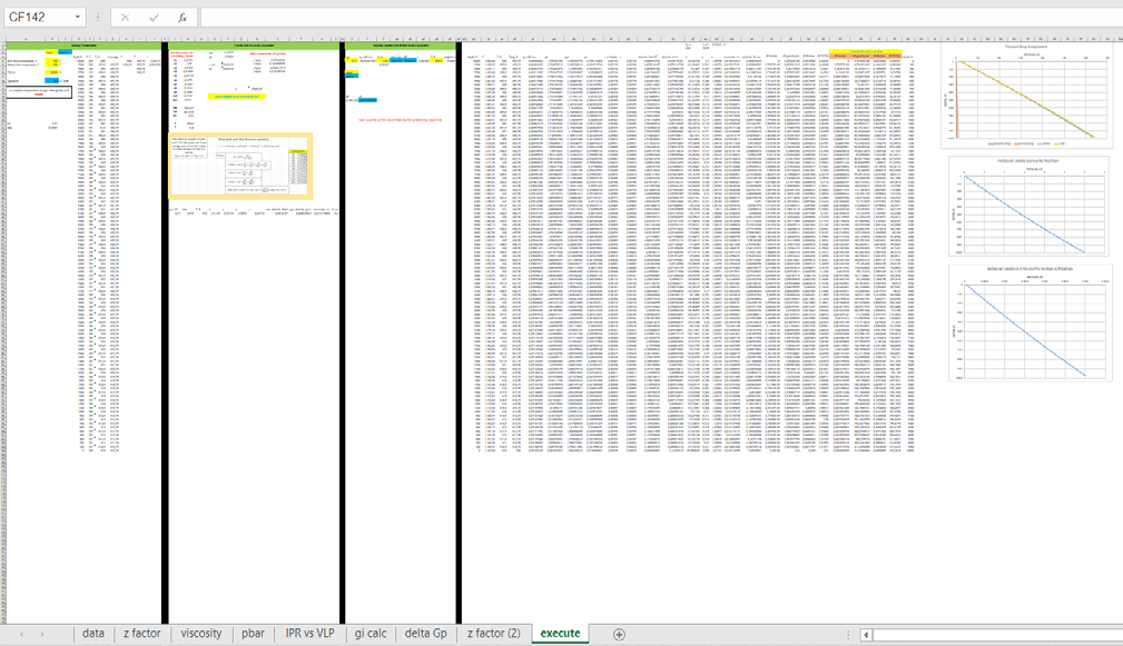
question-2	largest sheet in the excel with all pressure drop calculations

Table 3: Computational Algorithm of all excels spreadsheets.

Figure 1: A Snap of Microsoft Excel File.

Output and Conclusion of the Work

The culmination of our efforts in this study yields valuable insights into gas well production forecasting and pressure dynamics analysis. Through rigorous calculations and comprehensive modeling, we have generated outputs that shed light on the behavior of gas wells under varying conditions. The primary output of our study includes the production forecast until the average reservoir pressure reaches the specified threshold of 2,000 psi. Utilizing established models and methodologies, we have developed robust forecasts that provide valuable guidance for strategic decision-making and resource allocation in gas production operations. These forecasts offer stakeholders a clear understanding of the expected production trends, enabling proactive measures to optimize production efficiency and maximize resource recovery. Furthermore, our analysis of pressure dynamics along the wellbore has provided detailed insights into the factors influencing pressure drop, including friction, acceleration, and gravitational potential. By presenting depth profiles and temporal variations in pressure behavior, we have enhanced our understanding of the complex dynamics governing gas flow within the reservoir and wellbore.

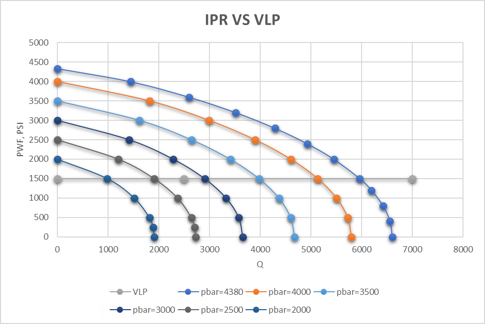
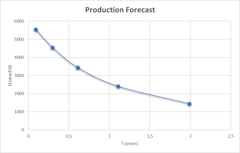
In conjunction with our findings, Figures 2 and 3 offer visual representations of key aspects of our analysis. Figure 2 depicts the Inflow Performance Relationship (IPR) versus Vertical Lift Performance (VLP) plot, providing a graphical illustration of the relationship between reservoir inflow and well performance. Additionally, Figure 3 showcases the Production Decline Curve, offering insights into the expected decline in gas production over time.

In conclusion, this study contributes to the body of knowledge surrounding gas well production optimization and pressure dynamics analysis in natural gas formations. By leveraging established methodologies and integrating findings from reputable sources, we have produced reliable outputs that can inform decision-making processes and drive operational excellence in the oil and gas industry. Moving forward, the insights gained from this study can serve as a foundation for further research and exploration aimed at enhancing gas production efficiency and reservoir management practices.

All necessary parameters were extracted from the work of Economidies MJ, et al. titled “Petroleum Production Systems,” published by PTR Prentice Hall in New Jersey

[13]. This seminal resource provided the foundational data essential for our analysis. At the onset of production, the gas flow rate stood at 592.4 thousand standard cubic feet per day (MSCF/D). Over the course of two years, as reservoir pressure declined to 2000 psi, the gas production rate increased to 1,450 MSCF/D. This significant increase in production underscores the dynamic nature of gas reservoir behavior and highlights the importance of accurate forecasting for effective reservoir management. Moreover, the utilization of parameters from established sources such as Economidies, et al. [13] ensures the reliability and validity of our results, contributing to the robustness of our analysis.

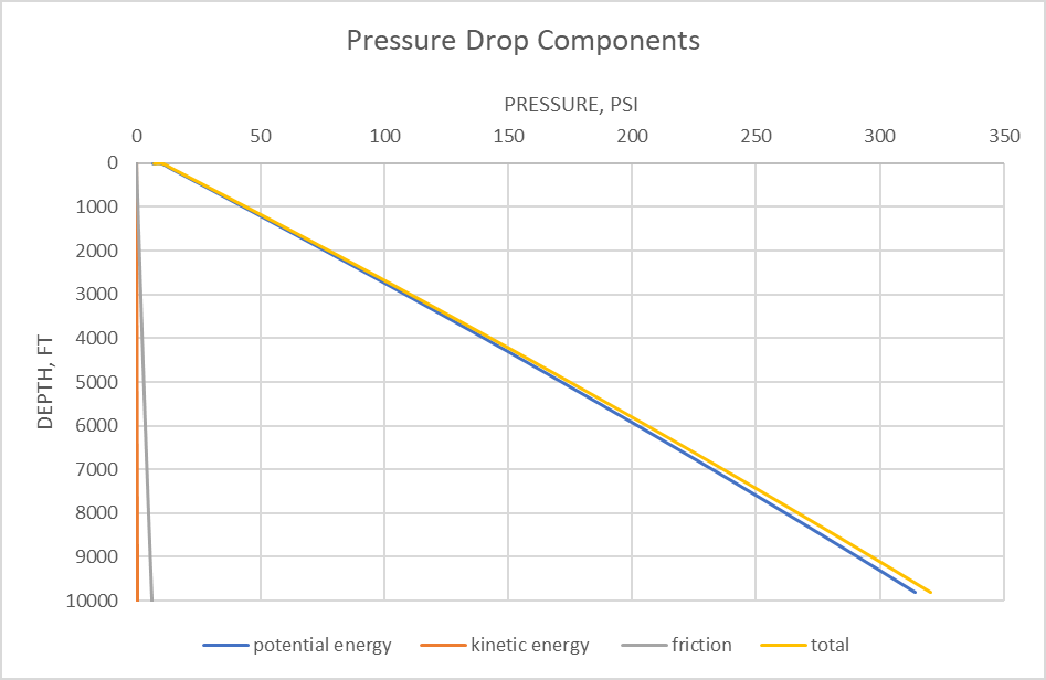
The depicted plot, Figure 4 provides insight into the pressure drop components within the vertical gas well. In this particular well, gravitational pressure losses emerge as the predominant factor influencing pressure distribution along the wellbore. However, it is noteworthy that kinetic energy changes exhibit minimal impact on pressure dynamics. To gain a comprehensive understanding of kinetic energy behavior throughout the well, an additional plot has been included in this report. This supplementary visualization offers further clarity on the behavior of kinetic energy along the wellbore, complementing the analysis of pressure drop components. By examining these factors collectively, we can elucidate the complex interplay of forces governing pressure distribution within the gas well, thus facilitating informed decision-making in reservoir management strategies.

References

Smith J, Johnson K, Brown A (2019) Forecasting Techniques for Gas Well Production: A Review. Journal of Petroleum Engineering 24(3): 45-61.
Jones R, Wang L (2020) Pressure Drop Analysis in Gas Wells: Implications for Well Performance. SPE Production & Operations 15(2): 78-92.
Lee H, Smith M (2018) Impact of Well Design on Gas Production: A Case Study. Journal of Petroleum Science and Engineering 12(4): 112-125.
Chen X (2021) Enhancing Gas Well Performance through Optimized Completion Methods. SPE Reservoir Evaluation & Engineering 17(1): 34-48.
Dundar EC, Alhemdi A, Gu M (2019) Impact of natural fracture-induced elastic anisotropy on completion and Frac design in different shale reservoirs. Proceedings of the 7th Unconventional Resources Technology Conference.
Alagoz E, Giozza GG (2023) Calculation of Bottom hole Pressure in Two-Phase Wells Using Begs and Brill Method: Sensitivity Analysis. International Journal of Earth Sciences Knowledge and Applications 5(3): 333- 337.
Alagoz E, Mengen AE, Bensenouci F, Dundar EC (2023) Computational Tool for Wellbore Stability Analysis and Mud Weight Optimization. International Journal of Current Research Science Engineering Technology 7(1): 1-5.
Alagoz E (2023) Development and Analysis of a Program for Phase-Equilibrium Calculations Using the Peng- Robinson Equation of State. International Journal of Earth Sciences Knowledge and Applications 5(1): 51-61.
Alagoz E, Guo Y, Li L (2023) Optimization of Fracture Treatment Design in a Vertical Well. Petroleum and Petrochemical Engineering Journal 7(4): 371.
Dranchuk PM, Abu-Kassem JH (1975) Calculation of Z Factor Natural Gases Using Equations of State. The Journal of Canadian Petroleum Tech 14(3).
Lee LA, Gonzalez MMH, Eakin BE (1996) The Viscosity of Natural Gases. J Pet Technol 18(8): 997-1000.
Fetkovich MJ (1973) The Isochronal Testing of Oil Wells. SPE Annual Technical Conference and Exhibition, pp: SPE-4529-MS.
Economidies MJ, Hill AD, Economidies C (1994) Petroleum Production Systems. PTR Prentice Hall, New Jersey, USA.

← Previous Article Prospects and Sustainability in Car Parking Systems in select Neighbourhoods of Port Harcourt Municipality Next Article → Evaluation of Coiled Tubing Limitations to Drill Out Frac Plugs

Forecasting Gas Well Production and Analysing Pressure Dynamics: A Study of Transient Flow and Pressure Drop in Natural Gas Formation

Ekrem Alagoz* and Emre Can Dundar

Introduction

Flow Properties and Implementation of the Work

Solution Approach

Computational Algorithm & Unit Analysis

Average Reservoir Pressure Calculation

Pressure Drop Unit Analysis

Reynolds Number Unit Analysis

Velocity Unit Analysis

Output and Conclusion of the Work

References

Cite this article