Thermal Conduction in Higher-Dimensional Sphere and Application to Fluid Rotation

Spherical Thermal Conduction Characterized by Advection and Diffusion

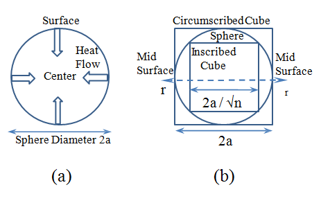
Heat Transfer between Adjacent $n$-Dimensional Spherical Shells: The inward thermal conduction of a sphere heated from the surface shown in Figure 1a is considered. The entire volume $nV$ and surface area $nS$ of the $n$-dimensional sphere with a radius of $a$ and the relation between $nV$ and $nS$ are given by [17].

$$nV = \frac{a^n \frac{n}{\pi^2}}{\Gamma\left(\frac{n}{2} + 1\right)}, nS = \frac{na^{n-1} \frac{n}{\pi^2}}{\Gamma\left(\frac{n}{2} + 1\right)}, nV = \int_0^a nSda,$$ (2.1)

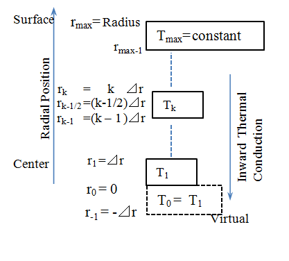
Where the function $\rho$ satisfies $\Gamma(n+1) = n\Gamma(n)$, and $\Gamma(1/2) = \pi^{1/2}$. The $n$-dimensional sphere is divided into a series of thin concentric shells with spherical symmetry and a thickness of $\Delta r$ as shown in Figure 2. Thermal conduction is calculated from the heat transfer between adjacent shells. The shell boundaries $r_k$ are subscripted with 0 to max such that $r_0 = 0.0$ and $r_{\max} = a$. The symbols $r_{k-1}, r_{k-1/2}$, and $r_k$ denote the inner radius $(k-1)\Delta r$, the central radius $(k-1/2)\Delta r$, and the outer radius $k\Delta r$ of the $k$-th shell, respectively. The number $k$ assigned to each shell coincides with that assigned to its outer boundary so that these positions are numbered from 1 to max. The temperatures of the shells are denoted $T_1$ to $T_{\max}$. The temperature of each shell is defined at the center of the shell, i.e., at $r = r_{k-1/2}$. Before $t = 0$, the temperatures of all shells $T_i$ ($i = 1 \rightarrow \max$) are set to zero as the initial condition. After $t = 0$, the temperature in the surface shell is maintained at a fixed temperature $T_s$, i.e., $T_{\max+1} = T_s$, and the inward thermal conduction transfers heat from the surface toward the center. The inward conduction requires central symmetry: $T_0 = T_1$. The volume $nV_k$ inner surface area $nS_k-1$, and outer surface area $nS_k$ of the $k$-th spherical shell in the $n$-dimensional sphere are derived from Equation (2.1) as

$$nV_k = \frac{\pi^2 \left( r_k^n - r_{k-1}^n \right)}{\Gamma\left(\frac{n}{2} + 1\right)}, nS_k = \frac{n\pi^2 r_k^{n-1}}{\Gamma\left(\frac{n}{2} + 1\right)}, nS_{k-1} = \frac{n\pi^2 r_{k-1}^{n-1}}{\Gamma\left(\frac{n}{2} + 1\right)}$$ (2.2)

In the $k$-th spherical shell ($k = 1 \rightarrow k_{\max}$), the volumetric heating is derived from the thermal conduction between adjacent shells. The progression in $t$ is denoted by the positive integer $m$. The present and next times are expressed using $m$ as $m\Delta t$ and $(m+1)\Delta t$, respectively, where $\Delta t$ is the minute time step. The heat influx $\Gamma_h$ is generated from the adjacent $(k+1)$-th shell to the $k$-th shell, which is proportional to the temperature gradient and surface area, expressed as $\Gamma_h = \lambda^n S_k\left(T_{k+1}^m - T_k^m\right)/\Delta r$, where $\lambda$ is the thermal conductivity, measured in watts per meter per degree Kelvin. The temperature $T_{k+1}^m$ of the $k$-th shell at the next time step $(m+1)\Delta t$ is determined by three terms at the present time step $m\Delta t$. The temperature of the $k$-th shell $T_{k+1}^m$, the heat transfer from the $(k+1)$-th shell $nS_k\left(T_{k+1}^m - T_k^m\right)/\Delta r$, and the heat transfer from the $(k-1)$-th shell $nS_k\left(T_{k+1}^m - T_k^m\right)/\Delta r$, which are expressed with a difference scheme with the aid of Equation (2.2) as

$$\rho C_p\left(r_k^n - r_{k-1}^n\right)\frac{T_{k+1}^m - T_k^m}{\Delta t} = \lambda n^k k^{n-1}\frac{T_{k+1}^m - T_k^m}{\Delta t} + \lambda n^k k^{n-1}\frac{T_{k+1}^m - T_k^m}{\Delta t}$$ (2.3)

Where $\rho C_p$ is the volumetric specific heat measured in joules per cubic meter per degree Kelvin. Equation (2.3) is arranged as a difference scheme as

$$\frac{T_{k+1}^m - T_k^m}{\Delta t} = x \frac{n}{r_k^n - r_{k-1}^n}\left(r_k^{n-1}\frac{T_{k+1}^m - T_k^m}{\Delta t} - r_{k-1}^{n-1}\frac{T_{k+1}^m - T_k^m}{\Delta t}\right)$$ (2.4)

Where $\chi$ is the thermal diffusivity $\lambda/(C_p\rho)$ measured in meters squared per second. Equation (2.4) is adequate for the numerical calculation of the thermal conduction of an $n$-dimensional sphere. The volume of the $k$-th spherical shell is proportional to $(r_k^n - r_{k-1}^n)$, which is approximated as $nr_{k-1}^n/2^{n-1}\Delta t$. Thus, Equation (2.4) converges to the following partial differential equation for infinitely small $\Delta r$ and $\Delta t$:

$$\frac{\partial T}{\partial t} = \chi \frac{1}{r^{n-1}}\frac{\partial r}{r^{n-1}}\frac{\partial T}{\partial r}$$ (2.5)

The form of Equation (2.5) is appropriate for numerical calculation using the difference scheme in Equation (2.4). Equation (2.5) can be equivalently converted into the following equation [10, 11, 12]:

$$\frac{\partial T}{\partial t} = \chi \left(\frac{\partial^2 T}{\partial r^2} + \frac{n-1}{r}\frac{\partial T}{\partial r}\right)$$ (2.6)

Equation (2.6) can compare the effects of the diffusion term $\partial^2 T/\partial r^2$ and the advection term $\partial T/\partial r$ appearing in the thermal conduction equation for $n \geq 2$, where the effect of the advection term becomes greater as $n$ increases, which is defined as a spherical geometry effect. Although thermal conduction mainly progresses by the planar heat transfer term ∂2_T_/ ∂r_2, ∂_T/∂r is related to spherical conversion and transfers heat in a different manner, as described in Secs. 3 and 4.

Click to enlarge

Click to enlarge

Convex Upward Temperature Profile Formed by the Advection Term

Planar heating from a single plane source located at r = 0, as shown in Figure 3a, is considered. The boundary conditions are expressed as follows:

$$ T (r, t < 0) = T _ {c} \mathrm {a n d} T (r = a, t \geq 0) = T _ {s}. \tag {2.7} $$ Before t = 0, both the surrounding volume and plane have a uniform temperature T(r, t) = T_c. After _t = 0, the temperature at the plane is maintained at a constant value of T_s(>_T_c). Consequently, the surrounding volume (_r > 0) is heated from the plane for t ≥ 0. Hereafter, it is assumed that T_c = 0 and _T_s = 1. The planar thermal conduction equation is derived from Equation (2.6) with for _n = 1 as

2 $$ \frac {\partial T}{\partial t} = \chi \frac {\partial^ {2} T}{\partial r ^ {2}} \tag {2.8} $$ By applying the boundary conditions in Equation (2.7) to Equation (2.8), the growth of the temperature profile is analytically derived as [1, 18, 19].

[ ] η η $$ 0 = T _ {s} \left[ 1 - e r f (\eta) \right], \quad \eta = - $$

s

$$ = \frac {2}{\sqrt {\pi}} \int_ {0} ^ {\eta} e ^ {- p ^ {2}} d p \left[ \approx \frac {2}{\sqrt {\pi}} \left(\eta - \frac {\eta^ {3}}{3} + \frac {\eta^ {5}}{1 0} - \frac {\eta^ {7}}{4 2} + \frac {\eta^ {9}}{2 1 6} + \dots\right) \right] $$

2 3 5 7 9 η η η η η η π π

erf e dp η

2 2 ( ) ----- 3

− p

10 42 216

0 The spatial differential on the right-hand side of Equation (2.8) contains only the diffusion term ∂2_T_/∂r_2. The temperature at any place except the boundary should increase with time, i.e., ∂_T/∂t > 0, in the case of planar heating. Therefore, planar heating always yields a convex downward temperature profile with no inflection points, i.e., ∂2_T_/∂r_2 > 0 for _r > 0. Although the diffusion term ∂2_T_/∂r_2 appears for both the planar and spherical geometries for _n ≥ 1, the advection term ∂T/∂r appears only for the spherical geometry for n ≥ 2, as shown in Equation (2.6). The elimination of the diffusion term ∂2_T_/∂_r_2 from Equation (2.6) yields the following hyperbolic equation:

1 0,for 1 (2.10) T n T n t r r χ ∂ − ∂ − ⋅ = ≥ ∂ ∂

The hyperbolic equation $\partial T/\partial t + u\partial T/\partial r = 0$ transfers heat with the heat transport velocity $u$. Thus, the temperature profile shifts in position with $u$. Equation (2.10) transfers heat from the planar heat source with the negative (centripetal) velocity $u = -\chi(n - 1)/r$ for $n \geq 2$. Thus, the step-like temperature profile formed at the surface just after $t = 0$ shifts in position toward the center with the centripetal velocity and forms a convex upward temperature profile. The temperature profile around the center is always convex downward. Therefore, the temperature profile for inward thermal conduction for $n \geq 2$ is composed of upward and downward convex curves and an inflection point.

**Fluid Torque Equations Equivalent to One-, Four- and Five-Dimensional Heating**

Fluid Rotation in a Cylinder Described as Four-Dimensional Spherical Heating: When the cylinder starts to rotate about the $z$ axis with a constant angular velocity $\Omega$ at $t = 0$, the cylindrical laminar flow layers rotate coaxially with the angular velocity $\omega(r)$ and diffuse from the surface cylindrical shell to the central axis. Finally, their velocity approaches $\Omega$. Each laminar flow layer is equivalent to the $k$-th cylindrical shell ($k = 1 \rightarrow k_{\text{max}}$) with the angular velocity $\omega_k$ and flow velocity $v_k = r_{k+1/2}\omega_k$. The flow grows owing to the torque acting between adjacent shells. The torque $\sigma$ acting on the $k$-th shell from the adjacent $(k + 1)$-th shell is expressed as the product of the radius $r_k$ as the length of the moment, the contacting surface area $2\pi r_k\Delta z$, and the velocity shear drag $\mu \left( r_{k\omega_k+1}^m - r_k\omega_k^m \right)/\Delta \rho$ and expressed as $\sigma = \mu r_k 2\pi r_k\Delta z \left( r_{k\omega_k+1}^m - r_k\omega_k^m \right)/\Delta r$, where $\Delta z$ is the length of the cylindrical shell. It should be noted that the flow velocity shear generated at the boundary radius $r = r_k$ originates from $r_k\omega_k+1^m - r_k\omega_k^m$; the velocity difference crossing the boundary because $\omega$ and the velocity shear are defined at the center of the shell at $r = r_{k+1/2}$ and the boundary between the shells at $r = r_k$, respectively. The total torque $N = N_k^{\text{upper}} + N_k^{\text{lower}}$ acting on the $k$-th shell is determined by the upper torque $N_k^{\text{upper}}$ from the $(k + 1)$-th shell and the lower torque $N_k^{\text{lower}}$ from the $(k - 1)$-th shell calculated at the present time step $m\Delta t$, where $N_k^{\text{upper}} = \mu r_k 2\pi r_k \left( r_{k\omega_k+1}^m - r_k\omega_k^m \right)/\Delta r$, and $N_k^{\text{lower}} = \mu r_k 1 2\pi r_{k-1} \left( r_{k-1}\omega_k+1^m - r_{k-1}\omega_k^m \right)/\Delta r$. Because the moment of inertia $I_k$ of the $k$-th shell rotating along the $z$ axis is $I_k = \rho \pi \left( r_k^2 - r_{k-1}^2 \right) r_k^2 \Delta z$, $\omega_k$ of the $k$-th shell is determined by a torque equation as

$$I_k \frac{\partial \omega_k}{\partial t} = N_k^{\text{upper}} + N_k^{\text{lower}} \tag{2.11}$$

Equation (2.11) is transformed into the difference scheme as follows, where $\omega_k^{m+1}$ at the next time step $(m + 1)\Delta t$ is determined by the quantities at the present time step $m\Delta t$:

$$\rho \left( \frac{2}{k} - \frac{2}{k-1} \right) r_k^2 \Delta z \frac{\omega_k^{m+1} - \omega_k^m}{Rt} r_k^2 \frac{1}{2}$$

$$= \mu 2\pi r_k \Delta z \frac{\left( r_k^{m+1} - r_k\omega_k^m \right)}{Rt} r_k + \mu 2\pi r_k-1 \Delta z \frac{\left( r_k^{m+1} - r_k\omega_k^m \right)}{Rt}$$

(2.12)

Using $r_k^2 - r_{k-1}^2 \approx jr_{k-1}/2^{j-1}\Delta r$, Equation (2.12) is transformed into

$$\rho \left( \frac{4}{k} - \frac{4}{k-1} \right) \frac{\omega_k^{m+1} - \omega_k^m}{Rt} = \mu 4\frac{3}{k} \frac{\left( \omega_k^{m+1} - \omega_k^m \right)}{Rt} + \mu 4\frac{3}{k-1} \frac{\left( \omega_k^{m+1} - \omega_k^m \right)}{Rt}$$

(2.13)

Equation (2.13) is equivalent to the thermal conduction of a four-dimensional sphere in Equation (2.3). The growth of the angular velocity profile is analogous to spherical heating from a surface for $n = 4$. The exchange of $T(r)$ with $\omega(r)$ and $\chi$ with $\nu = \mu/\rho$ in Equation (2.6) for $n = 4$ yields the growth shown in Figure 4(a4). The fluid between two coaxial cylinders having radii of $a$ and $b$ starts to rotate following the coaxial rotations of the inner and outer cylinders, where $\omega$ is $\Omega$ and $\omega_{\text{out}}$ at $r = a$ and $b$, respectively. After a growth period, the stationary angular velocity profile is derived from Equation (2.6) for $n = 4$ by setting $\partial/\partial t = 0$ as [6]

$$\omega = \frac{b^2}{\left( b^2 - a^2 \right)} \left[ \left( \Omega - \omega_{\text{out}} \right) \left( \frac{a}{r} \right)^2 - \Omega \left( \frac{a}{b} \right)^2 + \omega_{\text{out}} \right]$$

(2.14)

When the cylinder with a radius of $a$ rotates at $\omega = \Omega$ immersed in an infinitely wide static fluid, the angular velocity profile for $r \geq a$ is given as $\omega = \left( a/r \right)^2 \Omega$ by letting $b/a \rightarrow \infty$ and setting $\omega_{\text{out}} = 0$ in Equation (2.14). The force couple for the cylinder at a unit length for maintaining $\Omega$ is given as $4\pi a^2\mu\Omega$, which is derived from $2\pi a \times a \times \left( \partial(r/\omega) / \partial r \right)_{r=a}$.

Click to enlarge

Click to enlarge

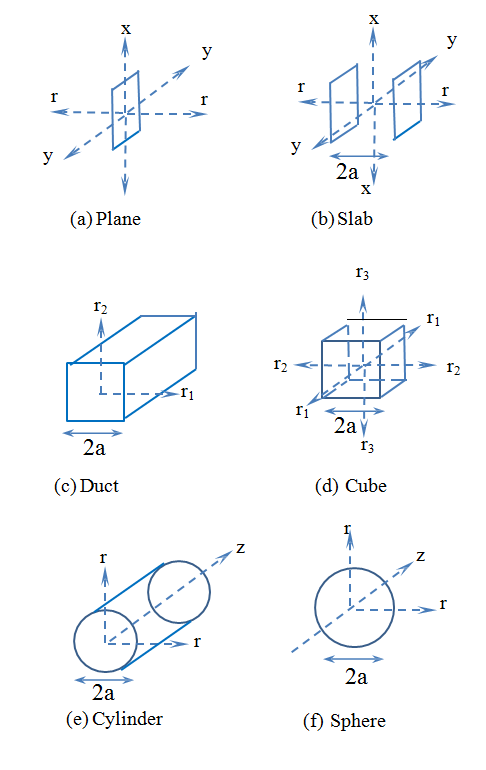
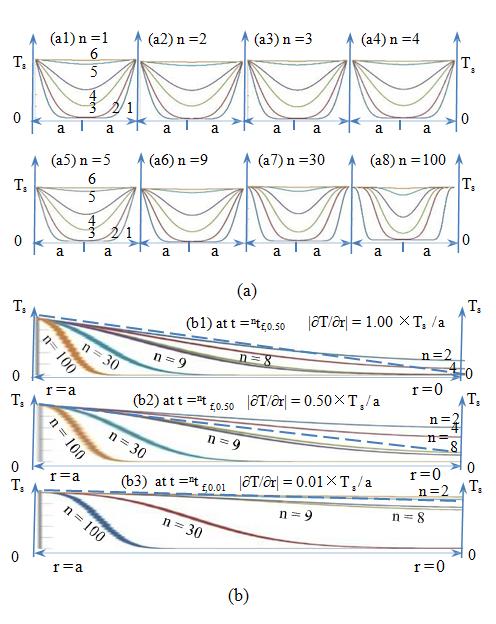
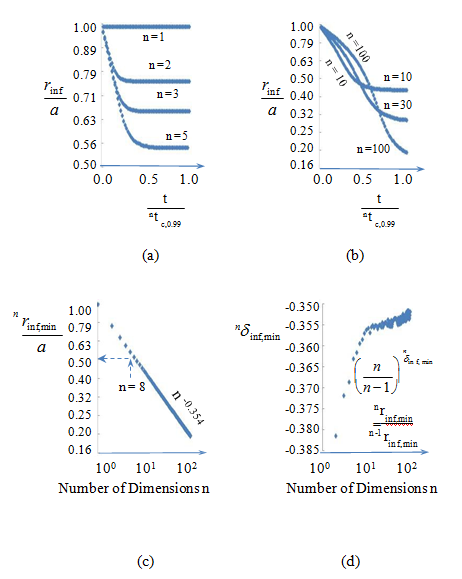
Figure 4: (a) Growth of temperature profiles due to inward thermal conduction of (a1) 1-, (a2) 2-, (a3) 3-, (a4) 4-, (a5) 5-, (a6) 9-, (a7) 30-, and (a8) 100- dimensional spheres heated from the surface. Because the temperature profile is the lowest at the center, the growth in the profile finally exhibits center filling. From t = 0 to t = nt_c0.99, six profile curves are plotted at _t = (1) nt_c0.01/2, (2) _nt_c0.01, (3) (_nt_c0.01 + _nt_c0.5)/2, (4) _nt_c0.5, (5) (_nt_c0.5 + _nt_c0.99)/2, and (6) _nt_c0.99. (b) Temperature profiles at the time when |∂_T/∂r|r=a decreases to (b1) 1.00_T_s/a, (b2) 0.50_T_s/a, and (b3) 0.01_T_s/a from ∞ at t = 0, where the surface temperature gradients |∂T/∂r|r=a are plotted as dotted straight lines. The six profiles at n = 2, 4, 8, 9, 30, and 100 are aligned from lowest to highest. Inflection points ∂2_T_/∂r_2 = 0 between the convex upward and downward parts are recognized for _n ≥ 2. The profile curves under the dashed lines distinguish the higher convex upward parts around the surface. Degree of upward convexity in the temperature profile can be visually recognized to be higher or lower according to n ≥ 9 or n ≤ 8, respectively.

Fluid Rotation in a Sphere Described as Five-Dimensional Spherical Heating

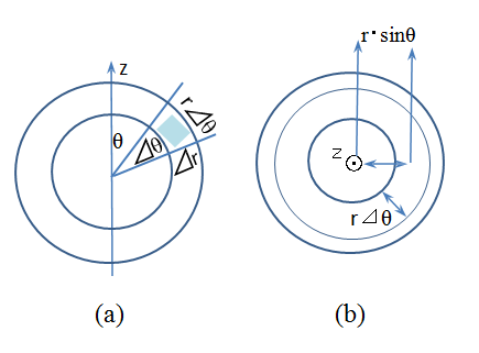
A rigid spherical shell with a diameter of 2a is immersed in a Newtonian fluid and has the coordinate system shown in Figure 3(f). The growth of the flow in the spherical shell is represented by laminar flow layers composed of thin concentric spherical shells. When the spherical shell starts to rotate along the z axis with a constant surface angular velocity of $\Omega$ at $t=0$, the spherical laminar flow layers rotate coaxially with the angular velocity $\omega(r)$ and diffuse to the center from the surface of the spherical shell. Finally, the spherical laminar flow layers approach $\Omega$. Each laminar flow layer is equivalent to the $k$-th spherical shell ($k=1 \rightarrow k_{\text{max}}$) with the angular velocity $\omega_k$ and radius $r_{k-1/2}$. The $k$-th spherical shell is divided into narrow rings with a similar azimuthal angle division $\Delta \theta$, as shown in Figure 5(a). The ring boundaries $\theta_i$ are subscripted with 0 to $j_{\text{max}}$ such that $\theta_0=0.0$ and $\theta_{\text{max}}=\pi$. The $j$-th ring for $(j-1)$ $\Delta \theta \leq \theta_j/\theta$ in the $k$-th shell for $(k-1)\Delta \theta \leq r \leq k\Delta r$ is considered. The angular velocity $\omega_{jk}$ of the ring is defined at the radial and azimuthal center of the ring, i.e., at $r=r_{k-1/2}$ and $\theta=j_{k-1/2}$. Because the cross section $S$ and the circumference $L$ of the ring are $S=\Delta r \times (r_{k-1/2}\Delta \theta)$ and $L=2\pi r_{k-1/2} \times \sin \theta_{j-1/2}$, respectively, as shown in Figure 5, the volume of the ring $V=LS$ is expressed as $V=2\pi r_{k-1/2} \times \sin \theta_{j-1/2} \times r_{k-1/2}\Delta \theta \Delta r$. Because the mass $M$ of the ring is $M=\rho V$, the moment of inertia $I_{jk}=M(r_{k-1/2} \times \sin \theta_{j-1/2})^2$, defined at the radial and azimuthal center of the ring, is given as $I_{jk}=\rho 2\pi r_{k-1/2} \times \sin 3\theta_{j-1/2}\Delta \theta \Delta r$. The flow velocity $v_k=\sin \theta_{j-1/2} \times r_{k-1/2} \times \omega_{jk}$ varies at each ring in the shell because $\theta_{j-1/2}$ varies at each ring. However, no torques are generated between the rings in the same spherical shell at $r=r_{k-1/2}$ because the angular velocity is the same for all $j(0 \leq j \leq j_{\text{max}})$ rings in the $k$-th spherical shell, i.e., $\omega_{jk}=\omega_k$. The flow grows owing to the torque acting between radially adjacent rings in a similar manner as the rotating cylindrical shell in Equation (2.11).

Because the torque $\sigma$ acting on the $j$-th (azimuthal) ring in the $k$-th (radial) shell from the radially adjacent $j$-th ring in the $(k+1)$-th shell is expressed as the product of the length of the rotation moment $\sin \theta_{j-1/2}r_k$ the contacting surface area $(2\pi \sin \theta_{j-1/2}r_k) \times (r_k\Delta \theta)$, and the velocity shear drag $\mu \Delta v_k/\Delta r=\mu(\sin \theta_{j-1/2}r_k \times \omega_{jk+1/2}-\sin \theta_{j-1/2}r_k \times \omega_{jk+1/2}-\sin \theta_{j-1/2}r_k \times \omega_{jk+1/2}-\sin \theta_{j-1/2}r_k \times \omega_{jk+1/2}-\sin \theta_{j-1/2}r_k \times \omega_{jk+1/2}-\sin \theta_{j-1/2}r_k \times \omega_{jk+1/2}-\sin \theta_{j-1/2}r_k \times \omega_{jk+1/2}-\sin \theta_{j-1/2}r_k \times \omega_{jk+1/2}-\sin \theta_{j-1/2}r_k \times \omega_{jk+1/2}-\sin \theta_{j-1/2}r_k \times \omega_{jk+1/2}-\sin \theta_{j-1/2}r_k \times \omega_{jk+1/2}-\sin \theta_{j-1/2}r_k \times \omega_{jk+1/2}-\sin \theta_{j-1/2}r_k \times \omega_{jk+1/2}-\sin \theta_{j-1/2}r_k \times \omega_{jk+1/2}-\sin \theta_{j-1/2}r_k \times \omega_{jk+1/2}-\sin \theta_{j-1/2}r_k \times \omega_{jk+1/2}-\sin \theta_{j-1/2}r_k \times \omega_{jk+1/2}-\sin \theta_{j-1/2}r_k \times \omega_{jk+1/2}-\sin \theta_{j-1/2}r_k \times \omega_{jk+1/2}-\sin \theta_{j-1/2}r_k \times \omega_{jk+1/2}-\sin \theta_{j-1/2}r_k \times \omega_{jk+1/2}-\sin \theta_{j-1/2}r_k \times \omega_{jk+1/2}-\sin \theta_{j-1/2}r_k \times \omega_{jk+1/2}-\sin \theta_{j-1/2}r_k \times \omega_{jk+1/2}-\sin \theta_{j-1/2}r_k \times \omega_{jk+1/2}-\sin \theta_{j-1/2}r_k \times \omega_{jk+1/2}-\sin \theta_{j-1/2}r_k \times \omega_{jk+1/2}-\sin \theta_{j-1/2}r_k \times \omega_{jk+1/2}-\sin \theta_{j-1/2}r_k \times \omega_{jk+1/2}-\sin \theta_{j-1/2}r_k \times \omega_{jk+1/2}-\sin \theta_{j-1/2}r_k \times \omega_{jk+1/2}-\sin \theta_{j-1/2}r_k \times \omega_{jk+1/2}-\sin \theta_{j-1/2}r_k \times \omega_{jk+1/2}-\sin \theta_{j-1/2}r_k \times \omega_{jk+1/2}-\sin \theta_{j-1/2}r_k \times \omega_{jk+1/2}-\sin \theta_{j-1/2}r_k \times \omega_{jk+1/2}-\sin \theta_{j-1/2}r_k \times \omega_{jk+1/2}-\sin \theta_{j-1/2}r_k \times \omega_{jk+1/2}-\sin \theta_{j-1/2}r_k \times \omega_{jk+1/2}-\sin \theta_{j-1/2}r_k \times \omega_{jk+1/2}-\sin \theta_{j-1/2}r_k \times \omega_{jk+1/2}-\sin \theta_{j-1/2}r_k \times \omega_{jk+1/2}-\sin \theta_{j-1/2}r_k \times \omega_{jk+1/2}-\sin \theta_{j-1/2}r_k \times \omega_{jk+1/2}-\sin \theta_{j-1/2}r_k \times \omega_{jk+1/2}-\sin \theta_{j-1/2}r_k \times \omega_{jk+1/2}-\sin \theta_{j-1/2}r_k \times \omega_{jk+1/2}-\sin \theta_{j-1/2}r_k \times \omega_{jk+1/2}-\sin \theta_{j-1/2}r_k \times \omega_{jk+1/2}-\sin \theta_{j-1/2}r_k \times \omega_{jk+1/2}-\sin \theta_{j-1/2}r_k \times \omega_{jk+1/2}-\sin \theta_{j-1/2}r_k \times \omega_{jk+1/2}-\sin \theta_{j-1/2}r_k \times \omega_{jk+1/2}-\sin \theta_{j-1/2}r_k \times \omega_{jk+1/2}-\sin \theta_{j-1/2}r_k \times \omega_{jk+1/2}-\sin \theta_{j-1/2}r_k \times \omega_{jk+1/2}-\sin \theta_{j-1/2}r_k \times \omega_{jk+1/2}-\sin \theta_{j-1/2}r_k \times \omega_{jk+1/2}-\sin \theta_{j-1/2}r_k \times \omega_{jk+1/2}-\sin \theta_{j-1/2}r_k \times \omega_{jk+1/2}-\sin \theta_{j-1/2}

When the sphere with a radius of a rotates at ω = Ω immersed in an infinitely wide static fluid, the angular velocity profile for r ≥ a is given as ω = (a/r)3Ω by letting b/a  ∞ and setting ω_out = 0 in Equation (2.17). The force couple for the sphere for maintaining Ω is given as 8π_a_3μΩ [7], which is derived from 2π_a_sinθ_aΔθ × a_sinθ × _a_sinθ(∂(_rω)/∂r|r=a).

Click to enlarge

Fluid Rotation in Two Discs Described as Slab Heating: The lamination of thin fluid discs with a radial diameter of 2_a_ and an axial thickness of Δz along the z axis constitutes a cylinder, as shown in Figure 3(e). The two surface discs at the ends of the cylinder are rigid discs located at z = ±h, where symmetry with respect to z = 0 is assumed. The discs surrounded by the two surface discs are the laminar flow layers of a Newtonian fluid, and the radial position r is defined by the distance from the z axis. It is assumed that no matter outside the cylinder for r > a exerts action on the fluid discs for r < a. When the two surface discs start to rotate about the z axis with a constant angular velocity Ω at t = 0, the laminar flow layer diffuses with an angular velocity of ω(z) from the surface discs to the center at z = 0, and the flow in the cylinder finally approaches a uniformly rotating flow with a surface angular velocity of Ω. The laminar flow layers are axially divided into concentric discs indexed by i (i = 1  i_max) with an axial thickness of Δ_z. The i-th disc is radially divided into concentric rings indexed by k (k = 1  k_max) with a radial thickness of Δ_r, as shown in Figure 2. The k-th ring for (k – 1)Δr ≤ r ≤ kΔr in the i-th disc for (i – 1)Δz ≤ z ≤ iΔz is considered. The angular velocity ωi,k of the ring is defined at the radial and axial center of the ring, i.e., at r = rk-1/2 and z = zi-1/2. Because the cross section S and the circumference L of the ring are S = ΔzΔr and L = 2πrk-1/2, respectively, as shown in Figure 5 at θ = π/2, the volume of the ring V = LS is derived as V = 2πrk-1/2ΔrΔz. Because the mass M of the ring is M = ρV, the moment of inertia Ik = Mrk-1/22, defined at the center of the ring, is given as Ik = ρ_2π_rk-1/23ΔrΔz. Although the flow velocity vk = rk-1/2_ω_i,k varies for each ring in the same disc, no torques are generated between the rings in the same disc because the angular velocity will be proven to be the same in the i-th disc, i.e., ωi,k = ωk. The flow grows owing to the rotation torque acting between axially adjacent rings according to Equation (2.11). Because the torque σ acting on the k-th (radial) ring in the i-th (axial) disc from the axially adjacent i-th ring in the (i + 1)-th disc is expressed as the product of the length of the rotation moment rk, the contacting surface area 2πrkΔr, and the velocity shear drag μΔvi,k/Δz =μ(rk-

1/2_ω_i+1,km – rk-1/2_ω_i,km)/Δz, σ = μrk-1/2 × 2πrk-1/2Δr(rk-1/2_ω_i+1,km – rk-1/2_ω_i,km)/Δz. The total torque N = Nk_upper + _Nk_lower acting on the _k-th ring in the i-th shell is determined by the upper torque Ni_upper from the (_i + 1)-th disc and the lower torque Ni_lower from the (_i – 1)-th disc calculated at the present time step mΔt, where Nk_upper = μr_k-1/2 × 2πrk-

1/2Δr(rk-1/2_ω_i+1,km – rk-1/2_ω_i,km)/Δz, and Nk_lower = μr_k-1/2 × 2πrk-

1/2Δr(rk-1/2_ω_i-1,km – rk-1/2_ω_i,km)/Δr. The angular velocity ωi,km+1of the k-th ring in the i-th disc at the next time step (m + 1)Δt is determined according to torque equation in Equation(2.11) as ( ) ( ) ( ) 1 m m m m m m $$ - r _ {k - 1}) \frac {\omega_ {i , k} ^ {m + 1} - \omega_ {i , k} ^ {m}}{t} = \mu \frac {\left(\omega_ {i , k + 1} ^ {m} - \omega_ {i , k} ^ {m}\right)}{z} + \mu \frac {\left(\omega_ {i , k - 1} ^ {m} - \omega_ {i , k} ^ {m}\right)}{z} $$ ω ω ω ω ω ω ρ μ μ , 1 , , 1 , , , (2.18) 1 i k i k i k i k i k i k r r k k t z z Where rk – rk-1 = Δr was used. Because time progression of ωi,k for any k-th ring in the same i-th disc is described by a torque equation similar to Equation (2.18), ωi,k is the same for all k (0 ≤ k ≤ k_max) rings in the _i-th disc, i.e., ωi,k = ωi. Equation (2.18) is equivalent to the slab heating of a volume surrounded by two parallel plates separated by 2_h_, as shown in Figure 3(b), i.e., the thermal conduction of a one-dimensional sphere in Equation (2.3). The growth of the angular velocity profile is analogous to slab heating from surface for n = 1 and shown in Figure 4(a1).

Specificity of the Diffusion Equation in the Geometry of an $n$-Dimensional Sphere

Analytical Formulae for the Heating Modes in One, Two, and Three Dimensions: Thermal conduction is restricted to the geometries of the heat sources and the surrounding volumes through which heat is transferred. The heat sources of a plane, a slab, an $n$-dimensional sphere, and a cube are shown in Figure 3. The origin of the radial coordinate $r$ is located at the center $r = 0$, and the surface of the volume is located at $r = a$. The centrosymmetric temperature profile $T(r, t)$ is measured in degrees Kelvin. The slab heating of a volume surrounded by two parallel plates separated by a distance of $2a$ is shown in Figure 3(b). The two positive directions of the $r$ axis originate at the origin and have opposite directions. The heating from cylindrical and spherical surfaces is shown in Figures 3(e) and 3(f), respectively, where the radii of the cylinder and sphere are $a$. The thermal conduction for the slab, cylinder, and sphere corresponds to the heating modes of one ($n = 1$), two ($n = 2$), and three ($n = 3$) -dimensional spheres, respectively, where $n$ is substituted into Equation (2.6). The boundary conditions are described by $r$ and the same for the three heating modes, as shown in Equation (2.7), where both the volume and surface have the uniform temperature $T(r, t) = T_c$ before $t = 0$, and the temperature at the surface is maintained at a constant value $T_s$ after $t = 0$. Consequently, the volume is heated from the surface at a constant temperature $T_s$ for $t \geq 0$.

By applying the boundary conditions

$$T(r \leq a, t < 0) = T_c$$ and $$T(r = a, t \geq 0) = T_s$$ (3.1)

where $T_c = 0$ and $T_s = 1$, Equation (2.6), the growth of the temperature profiles for one, two, and three-dimensional spheres is analytically derived as [10, 11, 12].

$$T(r, t) = T_s + 2\left(T_c - T_s\right) \sum_{n=1}^{\infty} \frac{(-1)^{n-1}}{a_n} \cos\left(\frac{r}{a}\right) \exp\left(-\frac{a^2}{2} \frac{x}{a^2}\right) a_n = n \frac{1}{2} \pi$$ (3.2a)

$$T(r, t) = T_s + 2\left(T_c - T_s\right) \sum_{n=1}^{\infty} \frac{(-1)^{n-1}}{a_n} \exp\left(-\frac{a^2}{2} \frac{x}{a^2}\right) J_0(b_n) = 0$$ (3.2b)

$$T(r, t) = T_s + 2\left(T_c - T_s\right) \sum_{n=1}^{\infty} \frac{(-1)^{n-1}}{a_n} \exp\left(-\frac{a^2}{2} \frac{x}{a^2}\right) J_0(b_1) = n \pi$$ (3.2c)

respectively, where $J_0$ and $J_1$ are the zeroth- and first-order Bessel functions, respectively; and $b_n$ ($>0$) satisfies $J_0(b_n) = 0$. Because Equation (3.2) involves exponentially decaying terms, the inward thermal conduction of an $n$-dimensional sphere finally approaches a flat temperature profile throughout the volume ($t \to \infty$), expressed as

$$T(r \leq a, t \to \infty) = T_S$$ (3.3)

which is obtained by solving Equation (2.6) and eliminating the time derivative $\partial/ \partial t$ on the left-hand side. The growing temperature profiles in Equations (3.2a), (3.2b), and (3.2c) are plotted in Figures 4(a1), 4(a2), and 4(a3), respectively, where the horizontal and vertical axes are the radial position $r$ and temperature $T$, respectively.

Time Period for Increasing the Center Temperature to the Surface Temperature

Since heat is transferred from the surface to the center, the temperature at the center is always the lowest until the end of the growth. By retaining the slowest exponential decay terms in Equation (3.2), the temperature profiles around the center at the final growth stage are given as

$$T = T_s + 2\left(T_c - T_s\right) \frac{2}{\pi} \cos\left(\frac{\pi}{2} \frac{r}{a}\right) \exp\left(-\frac{\pi^2}{4} \frac{x}{a^2}\right)$$ (3.4a)

$$T = T_s + 2\left(T_c - T_s\right) \frac{J_0\left(b_1 \frac{r}{a}\right)}{b_1 J_1(b_1)} \exp\left(-b_1^2 \frac{x}{a^2}\right) b_1 = 2.40$$ (3.4b)

$$T = T_s + 2\left(T_c - T_s\right) \frac{1}{\pi} \sin\left(\frac{\pi}{a}\right) \exp\left(-\pi^2 \frac{x}{a^2}\right)$$ (3.4c)

where $b_1 = 2.4$, $J_0(0) = 1$, $J_0(b_1) = 0$, and $J_1(b_1) = 0.519$. The three growth periods $1^{t_g}, 2^{t_g}$, and $3^{t_g}$ of the three heating modes assume that $1^{t_g} = 5 \times 4a^2/(\pi^2\chi)$, $2^{t_g} = 5 \times a^2/(2.4^2\chi)$, and $3^{t_g} = 5 \times a^2/(\pi^2\chi)^3$. When $t > 1^{t_g}$, $2^{t_g}$, and $3^{t_g}$, the slowest exponential decay terms in the three heating modes in Equations (3.4a), (3.4b), and (3.4c) become less than 0.0067, where exp $(-5) = 0.0067$ is used. Thus, $1^{t_g}$, $2^{t_g}$, and $3^{t_g}$ originating from the slowest exponential decay terms are the simplest evaluation of the growth period. In contrast, the growth period $n^{t_cf}$ is defined as the time when the temperature at the center $T_c = T(r = 0)$ is Nanomedicine & Nanotechnology Open Access

$$f(0.0 \leq f \leq 1.0) \text{ multiplied by the surface temperature } T_s, \text{ where } T_c = 0, \text{ as}$$

$$1_{t_c,f} = \frac{4}{\pi^2} \frac{a^2}{\chi} \log_e \frac{4}{\pi(1-f)}, \quad 2_{t_c,f} = \frac{1}{2.4^2} \frac{a^2}{\chi} \log_e \frac{2}{b_1 J_1(b_1)(1-f)}, \quad 3_{t_c,f} = \frac{1}{\pi^2} \frac{a^2}{\chi} \log_e \frac{4}{\pi(1-f)}$$

(3.5)

By setting $f = 0.99$ in Equation (3.5), $n_{t_c,0.99}$ could be obtained analytically for $n = 1, 2,$ and 3, where $1_{t_c,0.99}, 2_{t_c,0.99},$ and $3_{t_c,0.99}$ slightly deviate from $1_{t_g}, 2_{t_g},$ and $3_{t_g},$ respectively. $n_{t_g}$ and $n_{t_c,0.99}$ are compared as follows:

$$1_{t_g} = 2.03 \frac{a^2}{\chi} \left[ \frac{20}{\pi^2} \frac{a^2}{\chi} \right], \quad 2_{t_g} = 0.868 \frac{a^2}{\chi} \left[ \frac{5}{2.4^2} \frac{a^2}{\chi} \right], \quad 3_{t_g} = 0.507 \frac{a^2}{\chi} \left[ \frac{5}{\pi^2} \frac{a^2}{\chi} \right]$$

(3.6a)

$$1_{t_c,0.99} = 1.96 \frac{a^2}{\chi} \left[ \frac{4}{\pi^2} \frac{a^2}{\chi} \log_e \frac{400}{\pi} \right], \quad 2_{t_c,0.99} = 0.882 \frac{a^2}{\chi} \left[ \frac{1}{2.4^2} \frac{a^2}{\chi} \log_e \frac{200}{b_1 J_1(b_1)} \right], \quad 3_{t_c,0.99} = 0.490 \frac{a^2}{\chi} \left[ \frac{1}{\pi^2} \frac{a^2}{\chi} \log_e \frac{400}{\pi} \right]$$

(3.6b)

The steady flat temperature profiles for one-, two-, and three dimensional spheres are completed after $t = 1_{t_c,0.99}, 2_{t_c,0.99},$ and $3_{t_c,0.99},$ respectively.

$n$-Dimensional Cubes Inscribed within and Circumscribing an $n$-Dimensional Sphere: Although there are no analytical solutions for the inward thermal conduction of $n$-dimensional spheres heated from the surface for $n \geq 4,$ the growth period can be estimated through an extension of slab heating (one-dimension) to $n$ dimensions, i.e., the thermal conduction of an $n$-dimensional cube (hypercube) heated from the surface. A cube and its three-dimensional orthogonal coordinate system $r_1, r_2,$ and $r_3$ perpendicular to three planes are shown in Figure 3(d). The origins of $r_1, r_2,$ and $r_3$ are located at the center of the cube, and the radius $a$ of the cube is defined by the distance between the center and the plane. One- and two-dimensional cubes are a slab and square duct, as shown in Figures 3(b) and 3(c), respectively. In a similar manner, an $n$-dimensional cube described by the $n$-dimensional orthogonal coordinates $r_1, r_2, \dots, r_{n-1}, r_n$ is defined. The temperature $T$ inside the $n$-dimensional cube is expressed as $T(r_1, r_2, \dots, r_{n-1}, r_n t).$ The thermal conduction equation for the $n$-dimensional cube is an extension of Equation (2.8):

$$\frac{\partial T}{\partial t} = \chi \left( \frac{\partial^2 T}{\partial t_1^2} + \frac{\partial^2 T}{\partial t_2^2} + \dots + \frac{\partial^2 T}{\partial t_{n-1}^2} + \frac{\partial^2 T}{\partial t_n^2} \right)$$

(3.7)

The boundary conditions are similar to Equation (3.1) because $r_1, r_2, \dots, r_{n-1}, r_n$ are equivalent to $r.$ Moreover, the thermal conduction in a one-dimensional cube is similar to the slab heating in Equation (3.2a). The solution of Equation (3.7) is an extension of Equation (3.2a), which is a product of $n$ Fourier cosine functions of $r_1, \dots, r_n$ of which the exponential decay term involves $n.$ The temperature profile $T(r_1, r_2, \dots, r_{n-1}, r_n t)$ around the center at the final growth stage is derived as an extension of the slab heating in Equation (3.4a) to $n$ dimensions as

$$T = T_s + 2(T_c - T_s)\left(\frac{2}{\pi}\right)^n \exp\left(-\frac{\pi^2}{4} n \chi \frac{t}{a^2}\right)$$

(3.8)

The distance between two facing planes and the length of the diagonal are $2a$ and $2a\sqrt{n},$ respectively, for the $n$-dimensional cube. The relations between the cubes circumscribing and inscribed within a sphere with a radius of $a$ are shown in Figure 1(b), where the radii of the sphere and circumscribed cube are $a$ and that of the inscribed cube is $a/\sqrt{3}.$ In a similar manner, the radii $a_{\text{circ}}$ and $a_{\text{insc}}$ of the $n$-dimensional cube circumscribing and inscribed within an $n$-dimensional sphere with a radius of $a$ are determined to be $a_{\text{circ}} = a$ and $a_{\text{insc}} = a/n,$ respectively. $a_{\text{circ}}$ and $a_{\text{insc}}$ are substituted for $a$ in Equation (3.8) to evaluate the growth periods $n_{t_c}{\text{circ}}$ and $n{t_c}_{\text{insc}}$ for the inward thermal conduction of the circumscribed and inscribed $n$-dimensional cubes by retaining the slowest exponential decay terms in a similar manner as the derivation of $^1 t_g$ in Equation(3.6a) as

$$n_{t_{\text{circ}}} = \frac{1}{n} \frac{20}{\pi^2} \frac{a^2}{\chi} \quad \text{and} \quad n_{t_{\text{insc}}} = \frac{1}{n^2} \frac{20}{\pi^2} \frac{a^2}{\chi}, \quad n \geq 2 \quad (3.9)$$

The growth period $^n t_g$ of the thermal conduction of the $n$-dimensional sphere heated from the surface is shorter and longer than those of the $n$-dimensional circumscribed and inscribed cubes, respectively. Therefore, the range of $^n t_g$ of an $n$-dimensional sphere is determined according to the inequality $^n t_{\text{insc}} \leq^n t_g \leq^n t_{\text{circ}}$. Using Equation (3.9), the range of $^n t_g$ is expressed in terms of the power of $n$ as

$$\frac{1}{n^2} \frac{20}{\pi^2} \frac{a^2}{\chi} <^n t_g < \frac{1}{n^2} \frac{20}{\pi^2} \frac{a^2}{\chi}, \quad n \geq 2 \quad (3.10)$$

The growth periods evaluated from the extension of the slab heating in Equation (3.2a) by retaining the slowest exponential decay terms in Equations (3.4a) and (3.6a) lack rigorous precision, especially for higher values of $n$ because the temperature profile at the final growth stage should be calculated using the products of the lower and higher exponential decay terms in higher-dimensional cubes, in contrast to the slab heating calculated using only the lowest decay term in Equation (3.4a). However, the dependence of the growth period on $n$ can be estimated on the basis of the inequality in Equation (3.10). Because $^2 t_{\text{insc}} = 0.508a^2/\chi, ^2 t_{\text{circ}} = 1.02a^2/\chi$ and $^3 t_{\text{insc}} = 0.226a^2/\chi, ^3 t_{\text{circ}} = 0.677a^2/\chi$ in Equation(3.9), the analytically derived growth periods $^2 t_{c,0.99} = 0.882a^2/\chi$ and $^3 t_{c,0.99} = 0.490a^2/\chi$ for two- and three-dimensional spheres, respectively, as shown in Equation (3.6b), were found to be included in the inequality in Equation (3.10). Although the dependence of the growth period on $n$ can be quantitatively estimated from the fact that the surface-area-to-volume ratio $nS/nV$ of the $n$-dimensional sphere is proportional to $n/a$ from Equation (2.1), the qualitative evaluation of the dependence is given by Equation (3.10).

Numerical Accuracy Satisfying von Newman $n$ and Rightmyer’s Analysis and the CFL Condition

A numerical simulation of the thermal conduction can be performed using the difference scheme in Equation (2.4) and the boundary conditions in Equation (3.1) with $\chi = 1$ and $a = 1$. During the simulation, $T_k^{m+1}$ shifts to $T_k^m$ at the next time step. The thermal conduction equation in Equation (2.6) has both a diffusion term $\partial^2 T/\partial r^2$, as shown in Equation (2.8), and an advection term $\partial T/\partial r$, as shown in Equation (2.10) for $n \geq 2$. The diffusion equation in Equation (2.8) is restricted to the following stable simulation condition obtained by a von Neumann stability analysis [13, 14]:

$$t < \frac{(r)^2}{2\chi} \quad (4.1)$$

The hyperbolic equation in Equation (2.10) is restricted to the CFL condition [15, 16]. The CFL condition is expressed as $|u| < \Delta r/\Delta t$; that is, the heat transport velocity $|u| = \chi (n-1)/r$ appearing in the spherical thermal conduction equation should be less than the numerical grid velocity $\Delta r/\Delta t$ in the hyperbolic equation in Equation (2.10). Because $u$ is proportional to $r^1, |u|$ takes its maximum at $r = \Delta r$, which is the outer radius of the innermost shell. Thus, the CFL condition in Equation (2.10) should adopt $|u|$ as the maximum value of $|u| = \chi (n-1)/\Delta r$ and is expressed as

$$t < \frac{(r)^2}{(n-1)\chi} \quad (4.2)$$

Thus, $\Delta t$ for simulating Equation (2.10) should decrease as $n$ is increased, as shown in Equation (4.2), in contrast to $\Delta t$ for simulating Equation (2.8), which indicates no change with the increase in $n$, as shown in Equation (4.1). $\Delta t$ for simulating the planar diffusion equation in Equation (2.8) should satisfy only Equation (4.1), whereas that for the spherical diffusion equation in Equation (2.6) should satisfy both Equations (4.1) and (4.2). Therefore, the intersection between the two inequalities in Equations (4.1) and (4.2) is expressed as

$$t < \frac{(r)^2}{\xi\chi}, \quad \xi = A + B(n-1), A \geq 2.0 \text{ and } B \geq 1.0 \quad (4.3)$$

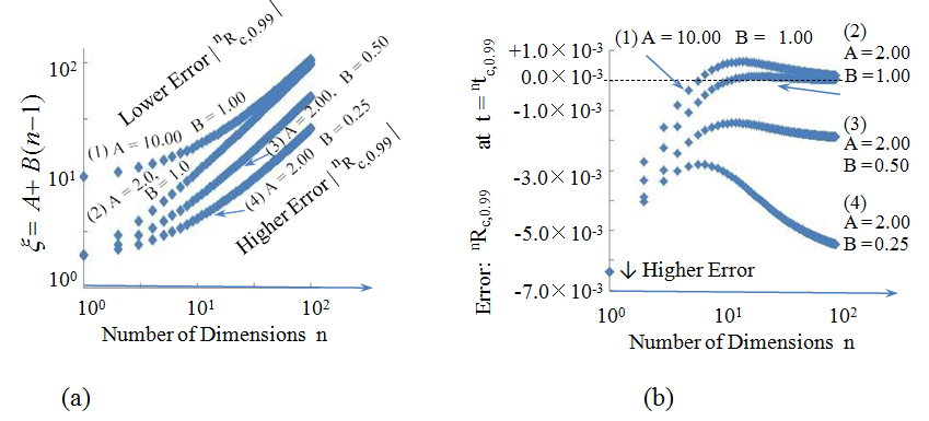
Equation (4.3) approaches Equations (4.1) and (4.2) as $n$ becomes low and high, respectively. The coefficients $A$ and $B$ in Equation (4.3) are derived from the stability condition in Equation (4.1) for the diffusion term in Equation (2.8) and that of Equation (4.2) for the advection term in Equation (2.10), respectively.

Even though Equation (4.3) is satisfied, the numerical accuracy should be evaluated from the balance of the heat influx entering at the surface and the increase in the heat energy of the entire volume. The heat influx $\Gamma_h$ is proportional to the temperature gradient at the surface $|\partial T/\partial r|{r=a}$ and the surface area $nS$, which is expressed as $\Gamma_h = \lambda n|\partial T/\partial r|{r=a}$ and measured in joules per second. Within $\Delta t$ at the m-th time step, $\Gamma_h$ and the heat increase in the entire volume of the sphere are balanced and expressed on the left- and right-hand sides, respectively, of the following equation:

$$\lambda^n S \Delta t \frac{T_{\max} - T_{\max-1}}{\Delta r} = \rho C_p \sum_{k=1}^{n} V_k \left( t_k^m - t_k^{m-1} \right)$$

where the superscript $m$, subscript $k$, and $nV_k$ are the m-th time step, the $k$-th spherical shell, and the volume of the $k$-th spherical shell, respectively. In Equation (4.4), $(T_{\max} - T_{\max-1})/\Delta r$ is $|\partial T/\partial r|_{r=a}$, and both sides have units of joules. Summing both sides of Equation (4.4) from $m = 1$ to $m = m$ leads to

$$\lambda^n S \Delta t \sum_{m=1}^{n} \frac{T_{\max} - T_{\max-1}}{\Delta r} = \rho C_p \sum_{k=1}^{n} V_k T_k^m - V_k T_k^{1}$$

If the time steps of 1 and $m + 1$ are the initial and final states, respectively, $T_k^1$ and $T_k^{m+1}$ are 0 and 1, respectively. Thermal conduction starts at $t = 0$. The period from $t = 0$ until $t = nT_c, 0.99$, defined as the time when the temperature at the center of the $n$-dimension sphere reaches 0.99 of the surface temperature, is the full profile completion period, which will be discussed in the next section. The summation on the left-hand side of Equation (4.5) should be continued at each time step from $t = 0$ until $t = nT_c, 0.99$. After $t = nT_c, 0.99$, the right-hand side of Equation (4.5) becomes $\rho C_p nV$ because $T_k^m (k = 1 \rightarrow k_{\max})$ is 1.0 and $\sum nV_k = nV$, as derived from Equation (2.2). The residual $nR_c, 0.99$ calculated from the difference between the left- and right-hand sides of Equation (4.5) at $t = nT_c, 0.99$ determines the numerical accuracy:

$$nR_c, 0.99 = \frac{n\chi t \sum_{m=1}^{n} \frac{T_{\max} - T_{\max-1}}{r}}{a}$$

Where $nS/nV = n/a$, derived from Equation (2.1), and $\chi = \lambda/(ρC_v)$ are used. A simulation result with a lower or higher $|nR_c, 0.99|$ indicates a higher or lower numerical accuracy, respectively.

Figure 6(a) shows the dependence of $\xi$ in Equation (4.3) on $A$, $B$, and $n$, where the horizontal and vertical axes are $\log_{10} n$ and $\xi$, respectively. There are four curves (1), (2), (3), and (4) with various values of $A$ and $B$ used in Equation (4.3): (1) $A = 10.0$, $B = 1.0$; (2) $A = 2.0$, $B = 1.0$; (3) $A = 2.0$, $B = 0.50$; and (4) $A = 2.0$, $B = 0.25$. With the shell thickness $\Delta r = a/500$, the dependence of $nR_c, 0.99$ in Equation (4.6) on $n$ is shown in Figure 6(b), where the horizontal and vertical axes are $\log_{10} n$ and $nR_c, 0.99$ ranging from $-7.0 \times 10^{-3}$ to $+1.0 \times 10^{-3}$, respectively. The four curves (1) $\rightarrow$ (4) adopt the same values of $A$ and $B$ in Figures 6(a) and (b). A higher $A$ and $B$ results in a higher $\xi$ in the upper part of Figure 6(a). Because $\Delta t$ is inversely proportional to $\xi$, as shown in Equation (4.3), a higher $\xi$ yields a lower $\Delta t$ and a higher accuracy with a lower $|nR_c, 0.99|$. Because analytical solutions have been obtained for $n \leq 3$, adequate values of $A$ and $B$ should be determined in order to restrict $|nR_c, 0.99|$ within $10^{-3}$ in the simulation for $n \geq 4$. When we adopt curve (2) ($A = 2.0$ and $B = 1.0$) in Figure 6, $|nR_c, 0.99|$ is restricted within $1.0 \times 10^{-3}$ from $n = 5$ to $n = 100$, while $|nR_c, 0.99| = 1.4 \times 10^{-3}$ at $n = 4$. When we adopt curve (1) ($A = 10.0$ and $B = 1.0$), the range of $|nR_c, 0.99|$ is restricted within $1.0 \times 10^{-3}$ from $n = 4$ to $n = 100$. Therefore, simulations from $n = 4-100$ will be conducted with $\Delta r = a/500$, $A = 10.0$, and $B = 1.0$ [curve (1)] hereafter because $|nR_c, 0.99|$ is restricted within $10^{-3}$ for $4 \leq n \leq 100$.

The lower $\Delta t$ created by $\xi$ in the upper part of Figure 6(a) yields a lower $|nR_c, 0.99|$ in Figure 6(b). Both of the stable simulation conditions in Equations (4.1) and (4.2) do not hold when $A < 2.0$ and $B < 1.0$. Thus, simulations conducted with $\xi$ existing below curve (2) ($A = 2.0$ and $B = 1.0$) in Figure 6(a) lead to a lower accuracy. The adoption of a lower $B$, as provided by curves (3) and (4) in Figure 6(a), results in a higher $|nR_c, 0.99|$ for $n \geq 4$ in Figure 6(b). Because curve (1) ($A = 10.0$ and $B = 1.00$) is above curve (2) ($A = 2.0$ and $B = 1.0$) in Figure 6(a), $|nR_c, 0.99|$ is reduced to $0.8 \times 10^{-3}$ on curve (1) for $n = 4$ in Figure 1(b). A decrease in $B$ compared to $B = 1.0$ yields a higher $|nR_c, 0.99|$ for $n \geq 4$, as shown in Figure 6(b). Because $\xi$ on curves (3) ($A = 2.0$ and $B = 0.50$) and (4) ($A = 2.0$ and $B = 0.25$) exists below curve (2) in Figure 6(a), $|nR_c, 0.99|$ on curves (3) and (4) exceeds $10^{-3}$ for $1 \leq n \leq 100$, as shown in Figure 6(b) while $|nR_c, 0.99|$ is restricted within $1.4 \times 10^{-3}$ for $4 \leq n \leq 100$ on.

curves (1) and (2). Because Equation (2.1) shows nS/nV = n/a, the heat transfer from the surface is more efficient for a higher n. As a result, the full profile completion period nt_c,0.99 becomes longer, and a larger number of time steps is required to complete the simulation for a lower _n. Thus, |nR_c,0.99| exceeds 10-3for _n ≤ 3, even for the adoption of the lowest Δt on curve (1) (A = 10.0 and B = 1.00). The higher |nR_c,0.99| for _n ≤ 3 causes no problems because numerical simulations should be conducted for n > 3. Simulations using Δt, where the CFL condition in Equation (4.2) does not hold, have been reported to yield meaningless divergent results [15, 16]. Current simulations based on the conditions on curves (3) (A = 2.0 and B = 0.50) and (4) (A = 2.0 and B = 0.25), where CFL condition does not hold, yielded convergent results, and |nR_c,0.99| on curves (3) and (4) in Figure 6(b) is comparatively greater than those on curves (1) and (2). The region where |_u| = χ (n – 1)/r exceeds Δr/Δt, i.e., the CFL condition in Equation (4.2) does not hold, exists within a limited narrow volume near the center where r/a << 1. Because |nR_c,0.99| is counted from the entire volume, the simulation was estimated to yield a convergent result, which |_nR_c,0.99| is restricted within 10-2, as shown in Figure 6(b), even though the condition _B < 1 on curves (3) and (4) are adopted. However, the current simulations with A < 2.0 and B = 0, where both Equations (4.1) and (4.2) do not hold, definitely yielded meaningless divergent results because the stable simulation condition in Equation (4.1) should hold in the entire volume of the n-dimensional sphere, even though CFL condition does not hold only near the center.

Click to enlarge

Initial Surface Influx Period and Final Center Filling Period

The temperature profile grows from the surface and finally completes a stationary flat temperature profile. The heat influx is proportional to the temperature gradient at surface|∂T/∂r|r=a, which is higher in the initial growth stage. Because the temperature T_o at the center _r = 0 is always the lowest, as shown in Figure 4, the final growth stage has a center filling period during which the center temperature increases to the surface temperature level. Thus, the growth of the profile is divided into the initial high surface influx stage and the final center filling stage, which are discriminated by the magnitude of $\Delta T/\partial r|{=a}$ and $\Delta T{s-c} = (T_s - T_o)/T_s$, where $T_s - T_o$ is the difference in the temperatures at the surface and center. Three center filling periods $n_{t_{c,0.99}}$, $n_{t_{c,0.50}}$ and $n_{t_{c,0.01}}$ were defined as the times when $T_o$ reaches 0.997$T_s$, 0.50$T_s$, and 0.017$T_s$, respectively, $n_{t_{c,0.99}}$, $n_{t_{c,0.50}}$, and $n_{t_{c,0.01}}$ were found to decrease with $n$, as shown in Figure 7(a), where the horizontal and vertical axes are $\log_{10}(n)$ and $\log_{10}(n_{t_{c,0.99}})$, $\log_{10}(n_{t_{c,0.50}})$, and $\log_{10}(n_{t_{c,0.01}})$, respectively. Setting $a = \chi = 1$, the center filling periods $1_{t_{c,0.99}} = 1.96$, $2_{t_{c,0.99}} = 0.882$, and $3_{t_{c,0.99}} = 0.490$ are analytically determined from Equation (3.5) with $f = 0.99$. Equation (3.5) with $f = 0.50$ yielded $1_{t_{c,0.50}} = 0.379$, $2_{t_{c,0.50}} = 0.203$, and $3_{t_{c,0.50}} = 0.0947$, and that with $f = 0.01$ yielded $1_{t_{c,0.01}} = 0.102$, $2_{t_{c,0.01}} = 0.0840$, and $3_{t_{c,0.01}} = 0.025$. $n_{t_{c,0.99}}$, $n_{t_{c,0.50}}$, and $n_{t_{c,0.01}}$ for $n \leq 3$ are involved in the numerical simulation from $n = 1$ to $n = 100$ in Figure 7(a). Because the final steady flat profile is almost completed at the center after $t = n_{t_{c,0.99}}$ at each $n_{t_{c,0.99}}$ is defined as the full profile completion period, and all time scales will be normalized by $n_{t_{c,0.99}}$ at each $n$ hereafter. The growth of the temperature profile of (a) 1-, (b) 2-, (c) 3-, (d) 4-, (e) 5-, (f) 9-, (g) 30-, and (h) 100-dimensional spheres are shown in Figure 4. During the full completion period from $t = 0$ to $t = n_{t_{c,0.99}}$, the profile curves are displayed at the following six times: $t = (1) n_{t_{c,0.01}}/2$, $(2) n_{t_{c,0.01}}/3$, $(3) n_{t_{c,0.01}} + n_{t_{c,0.50}}/2$, $(4) n_{t_{c,0.50}}/5$, $(5) n_{t_{c,0.50}} + n_{t_{c,0.99}}/2$, and $(6) n_{t_{c,0.99}}$. The decreases in $n_{t_{c,0.99}}$, $n_{t_{c,0.50}}$, and $n_{t_{c,0.01}}$ with the increase in $n$, in comparison with planar diffusion at $n = 1$, are due to the effects of the spherical geometry because the surface-to-volume ratio is proportional to $n(n^2/S)/V = n/a$. Figure 4 shows $\Delta T_{s-c} = (T_s - T_o)/T_s$ decreases with time. The degree of the center filling is numerically evaluated by $\Delta T_{s-c}$. For $n = 1, 10, 50,$ and 100, the changes in $\Delta T_{s-c}$ with time are compared in Figure 7(b), where the horizontal and vertical axes are the time normalized by $n_{t_{c,0.99}}$ and $\log_{10}(\Delta T_{s-c})$, respectively. The analytical solutions of Equation (3.4) indicate that $\Delta T_{s-c}$ decreases exponentially with time for $n \leq 3$. Although $\Delta T_{s-c}$ for $n = 1$ decreases exponentially with time (a linear curve), it is a convex upward curve for $n \geq 2$, and the curvature is visually recognized to be distinct for $n \geq 9$. Thus, the center filling period was considered to be biased to the final stage in the full profile completion period $n_{t_{c,0.99}}$ for $n \geq 9$.

The bias of the center filling period to the final stage is evaluated by the ratios $n_{t_{c,0.50}}/n_{t_{c,0.99}}$ and $n_{t_{c,0.01}}/n_{t_{c,0.99}}$, which are plotted as a function of $n$ in Figure 7(c), where the horizontal and vertical axes are $\log_{10}(n)$ and $n_{t_{c,0.50}}/n_{t_{c,0.99}}$, respectively. These two ratios were found to approach asymptotic lines for $n \geq 9$ and show that the center filling period is biased to the final stage with the increase of $n$. The time for $T_{s-c}$ to reach 0.50$T_{s}$ requires 70% of the full profile completion period $n_{t_{c,0.99}}$ at $n = 100$, whereas that requires 20% of $n_{t_{c,0.99}}$ at $n = 1$. The time for $T_{s-c}$ to reach 0.01 $T_{s}$ requires 50% of $n_{t_{c,0.99}}$ at $n = 100$, while that requires only 2% of $n_{t_{c,0.99}}$ at $n = 1$. Thus, the center filling period was determined to be biased to the final stage with the increase in $n$. Because there is a linear relation between $\log_{10}(n)$ and $\log_{10}(n_{t_{c,0.99}})$ in Figure 7(a), $n_{t_{c,0.99}}$ is expected to be proportional to $n$ to the power index of $n_{t_{c,0.99}}$. Because $n_{t_{c,0.99}}$ was calculated from $n_{t_{c,0.99}}/n^{1}n_{t_{c,0.99}} = n^8/(n-1)^8$, i.e., $n_{t_{c,0.99}} = \log_{10}(n_{t_{c,0.99}}/n^{1}n_{t_{c,0.99}})/\log_{10}(n/(n-1))$, $n_{t_{c,0.99}}$ cannot be defined for one dimension. The dependence of $n_{t_{c,0.99}}$ on $n$ is plotted in Figure 7(d), where the horizontal and vertical axes are $\log_{10}(n)$ and $n_{t_{c,0.99}}$ respectively. The power indices $2^{n_{t_{c,0.99}}} = -1.159$ and $3^{n_{t_{c,0.99}}} = -1.213$ are calculated from the analytical solutions of Equation (3.4) and are in agreement with the numerical results. Because the rate of change in $[n^{2}n_{t_{c,0.99}}]$ remains within 12% from $n = 2$ to $n = 100$, a power law was determined, wherein $n_{t_{c,0.99}}$ was proportional to $n$ to the power of $n_{t_{c,0.99}}$. The numerically determined values of $4^{n_{t_{c,0.99}}}$ and $5^{n_{t_{c,0.99}}}$ are $-1.241$ and $-1.259$, respectively. The power index $n_{t_{c,0.99}}$ was assumed to be $-1.25$, which is the average of $4^{n_{t_{c,0.99}}}$ and $5^{n_{t_{c,0.99}}}$. Therefore, $n_{t_{c,0.99}}$ affected by the spherical geometry was found to be expressed as a power law in Equation (4.7a). The reasons to adopt the average of $4^{n_{t_{c,0.99}}}$ and $5^{n_{t_{c,0.99}}}$ are as follows. The average value is almost the center value from $n = 1$ to $n = 100$, the growth periods for $n = 4$ and 5 can be verified through a fluid rotation measurement, and the average of the two values has more reproducibility than a least-squares fitting. In a previous study, $n_{t_{c,0.99}}$ was assumed to be $-1.24$ from a least-squares fitting from $n = 1$ to 100 [12]. Because the surface-to-volume ratio increases with $n$, the influx efficiency increases with $n$. Thus, another relation between $n_{t_{c,0.9

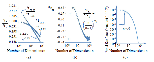
The heat influx proportional to the temperature gradient at the surface $|\partial T/\partial r|{r=a}$ begins at an infinitely large value and approaches zero after $t = n t{c,0.99}$. The decrease in $|\partial T/\partial r|{r=a}$ with time $t$ for $n = 1, 10, 50,$ and 100 are compared in Figure 8(a), where the horizontal and vertical axes are the time normalized by $n t{c,0.99}$ and $\log_{10}|\partial T/\partial r|{r=a}$ respectively. From the analytical solutions of Equation (3.2), $|\partial T/\partial r|{r=a}$ is expected to decrease exponentially with the time for $1 \leq n \leq 3$. Numerical simulations for $4 \leq n \leq 100$ show that $|\partial T/\partial r|{r=a}$ also decreases exponentially with the time. Although $|\partial T/\partial r|{r=a}$ always decreases exponentially with the time, the decrease in $\Delta T_{s,c}$ is biased to the final stage for higher $n$ while $\Delta T_{s,c}$ decreases exponentially with time for $n \leq 3,$ as shown in Figure 7(b). Because $|\partial T/\partial r|{r=a}$ is higher at the initial stage, the measurement of $|\partial T/\partial r|{r=a}$ in terms of $T_s/a$ characterizes the inflow period. Three influx periods $n t_{1.00}, n t_{0.50},$ and $n t_{0.01}$ were defined as the times when $|\partial T/\partial r|{r=a}$ reaches $1.0 T_s/a,$ $0.5 T_s/a,$ and $0.01 T_s/a,$ respectively. $n t{1.00}, n t_{0.50},$ and $n t_{0.01}$ decrease with $n,$ as shown in Figure 8(b), where the horizontal and vertical axes are $\log_{10}(n)$ and $\log_{10}(n t_{1.00}),$ $\log_{10}(n t_{0.50}),$ and $\log_{10}(n t_{0.01})$, respectively. The three influx periods for $1 \leq n \leq 3$ can be derived analytically in a similar manner as Equation (3.6b). Because there is a linear relation between $\log_{10}(n)$ and $\log_{10}(n t_{0.01})$ in Figure 8(b), $n t_{0.01}$ is expected to be proportional to $n$ to the power index of $n t_{0.01}.$ Because $n t_{0.01}$ was calculated from $n t_{1.00} n t_{0.01} = n^8/(n - 1)^8,$ i.e., $n t_{0.01} = \log_{10}(n t_{0.01})/\log_{10}(n/(n - 1)),$ $n t_{0.01}$ cannot be defined for one dimension. The dependence of $n t_{0.01}$ on $n$ is plotted in Figure 8(c), where the horizontal and vertical axes are $\log_{10}(n)$ and $n t_{0.01},$ respectively. The rate of change in $n t_{0.01}$ exceeds 50% because $2 t_{0.01} = -1.22$ at $n = 2$ and $100 t_{0.01} = -1.78$ at $n = 100.$ $n t_{0.01}$ was assumed to be $-1.5,$ which is the average of $2 t_{0.01}$ and $100 t_{0.01}.$ Although the heat influx is higher at the initial stage, the stationary flat profile is almost completed after $t = n t_{c,0.99}$ in a similar manner as the full profile completion after $t = n t_{c,0.99}.$ Therefore, $n t_{c,0.99}$ was found to be expressed as a power law as follows:

$$n t_{f,0.01} = n^{-1.50} \frac{21.2}{\pi^2} \frac{a^2}{\chi}$$

Where $21.2 = 4 \log_e(200),$ which is derived from $|\partial T/\partial r|{r=a}$ in the analytical solution of Equation (3.4a). Equation (4.8) is supported by Equation (4.7c) in a similar manner as $n t{c,0.99}.$ Considering the finding that the rate of change in $n t_{c,0.99}$ exceeds 50%, it was concluded that the power law of $n t_{c,0.01}$ in Equation (4.8) is inferior to that of $n t_{c,0.99}$ in Equation (4.7a). There is an essential difference between Figure 7(b) and Figure 8(a); that is, the center filling and surface influx obey spherical and planar geometries, respectively. $n t_{c,0.99}$ can be well-described by the concise power law of $n$ in Figure 7(d) and Equation (4.7c) owing to the effect of the spherical geometry at the center, whereas $n t_{c,0.99}$ cannot be well-described by the concise power law of $n$ in Figure 8(c) and Equation (4.8) owing to the insufficient effect of the spherical geometry on the surface.

$T_o$ increases exponentially with the time at the full profile completion period at $t = n t_{c,0.99},$ as shown in Figure 7(b). $|\partial T/\partial r|{r=a}$ almost always decreases exponentially with time, as shown in Figure 8(a). Thus, the coefficient $k{cent,fin}$ representing the exponential increase in $T_o$ and the coefficient $k_{surf,fin}$ representing the exponential decrease in $|\partial T/\partial r|{r=a}$ are respectively defined in the difference scheme at $t = n t{c,0.99}$ as follows:

$$T_0^m \cdot e^{+k_{cent,fin} \Delta t} = T_0^{m+1}$$

$$\left( \frac{T_0^m - T_0^{m-1}}{\Delta r} \right) \cdot e^{-k_{surf,fin} t} = \left( \frac{T_0^{m+1} - T_0^{m-1}}{\Delta r} \right)$$

Where $m + 1$ and $m$ denote the final time step and the time step before the final time step, respectively. The dependencies of $k_{cent,fin}$ and $k_{surf,fin}$ on $n$ are plotted in Figure 8(d), where the horizontal and vertical axes are $n$ and the coefficients, respectively. Because there is almost a linear relation between $\log_{10}(n)$ and $\log_{10}(k_{cent,fin})$ and $\log_{10}(k_{surf,fin})$, $k_{cent,fin}$ and $k_{surf,fin}$ can be described by power laws as

$$k_{cent,fin} = 2.46 \times 10^{-0} \cdot n^{1.57}$$

$$k_{surf,fin} = 2.45 \times 10^{-2} \cdot n^{1.51}$$

$$k_{surf,fin} = 2.45 \times 10^{-2} \cdot n^{1.51}$$

The powers of 1.57 and 1.51 for k_cent,fin and _k_surf,fin in Equation (4.10) are similar, where both |∂_T/∂r|r=a and T_s – _T_o are close to zero at _t = nt_c,0.99. Although |∂_T/∂r|r=a decreases exponentially with the time in a similar manner as planar thermal conduction, Equation (4.10) indicates that k_cent,fin and _k_surf,fin change with _n with similar power indices. Therefore, it was concluded that the changes in the temperature profiles with the time at both the surface and center at t = nt_c,0.99 were determined in an equivalent manner by the effect of the spherical geometry indicated by _n – 1 despite the effect of the planar geometry on the surface.

Click to enlarge

Click to enlarge

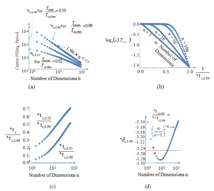
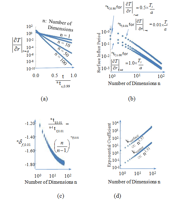
Figure 8: (a) The absolute value of the temperature gradient at the surface |∂T/∂r|r=a is +∞ at t = 0 and decreases exponentially with the time from n = 1 to n = 100, where the surface heat influx is proportional to |∂T/∂r|r=a. (b) After the three influx periods of nt_f,0.01, _nt_f,0.50, and _nt_f,1.00, |∂_T/∂r|r=a decreases from ∞ at t = 0 to 0.01_T_c/a, 0.50_T_c/a, and 1.00_T_c/a, respectively. The three influx periods decrease with n. The temperature profile is almost flat around the surface (r = a) after t ≥ nt_f,0.01. (c) The influx period _nt_f,0.01 is proportional to _n to the power index of nδf,0.01. (d) The coefficients of k_surf,fin representing the exponential decrease in |∂_T/∂/r|r=a with the time and k_cent,fin representing the exponential increase in _T(r = 0) with the time depend on n as n_1.57and _n_1.51, respectively at _t = nt_c,0.99. Motion of the Inflection Point and the Degree of Upward Convexity in the Profile The temperature profile for planar or slab heating exhibits a convex downward curve, as discussed in Sec. 2. Higher-dimensional spherical heating exhibits both convex upward and downward curves owing to the advection term in the thermal conduction equation in Equation (2.6). The inflection point ∂2_T/∂r_2 = 0 between the convex upward and downward profiles is created at the surface of the sphere at _t = 0 and is then shifted toward the center after t = 0. The changes in the radial position of the inflection point with the time for n = 1, 2, 3, and 5 and n = 10, 30, and 100 are shown in Figures 9(a) and (b), respectively, where the horizontal and vertical axes are t and log10(r/a), respectively, and r/a is the radial-position-to-radius ratio. Centripetal motion of the inflection point was found to occur intensively during the initial stage (0 ≤ t< nt_c,0.99/2) for _n ≤ 7 (Figure 9(a)) and continued to the final stage (nt_c,0.99/2 ≤ _t ≤ nt_c,0.99) for _n ≥ 8 (Figure 9(b)). The inflection point was found to reach the closest approaching distance nr_inf,min from the center at _t = nt_c,0.99. In the case of planar heating for _n = 1, 1_r_inf,min/a = 1 because no inflection points are created (Figure 9(a)). The relation between r_inf,min/_a and n is shown in Figure 9(c), where the horizontal and vertical axes are log10(n) and log10(nr_inf,min/_a), respectively. nr_inf,min/_a decreases from 1_r_inf,min/a = 1.0 at n = 1 to 100_r_inf,min/a = 0.2 at n = 100, and there is a linear relation between log10(n) and log10(nr_inf,min/_a). Thus, nr_inf,min/_a is expected to be proportional to n to the power index of nδinf,min. nδinf,min was calculated from nδinf,min = log10(nr_inf,min/_n-1_r_inf,min)/log10{n/(n – 1)}. The dependence of nδinf,min on n is plotted in Figure 8(d), where the horizontal and vertical axes are log10(n) and nδinf,min, respectively. Although nδinf,min changes with n from –0.382 to –0.355 for 2 ≤ n ≤ 9, nδinf,min remains around –0.354 for 10 ≤ n ≤ 100. Because the rate of change in |nδinf,min| remains within 9% from n = 2 to n = 100, a power law was determined, wherein n_rinf,min/_a was proportional to n to the power of nδinf,min = –0.354. Therefore, r_inf,min/_a affected by the spherical geometry was found be described by the following power law:

Because 0.5 = 7.08-0.354, the inflection point nr_inf,min reaches within half of the radius _a from the center for n ≥ 8. Thus, the degree of upward convexity is determined to be distinct for n ≥ 8. The advection term (n – 1)(1/r)(∂T/∂r) in Equation (2.6) generates the convex upward part in the profile curve for n ≥ 2, adding to the diffusion term (∂2_T_/∂r_2) that causes the convex downward profile. Although an inflection point is always generated for _n ≥ 2, the degree of upward convexity is distinct for n ≥ 9, as shown in Figures 4(a6)–(a8), and not distinct for 2 ≤ n ≤ 5, as shown in Figures 4(a2)–(a5). The degree of upward convexity is compared with profiles for n = 2, 4, 8, 9, 30, and 100 at the times when t = nt_f,1.00(|∂_T/∂r|r=a = 1.0_T_s/a), t = nt_f,0.50(|∂_T/∂r|r=a = 0.5_T_s/a), and t = nt_f,0.01(|∂_T/∂r|r=a = 0.01_T_s/a) in Figures 4(b1), 4(b2), and 4(b3), respectively, where the horizontal and vertical axes are the radial position from r = a to r = 0 and T, respectively. The temperature T_o’ at the center is defined as _T_o’ = _T_s – |∂_T/∂r|r=aa; that is, the temperature decreases from the surface while maintaining the same temperature gradient at the surface |∂T/∂r|r=a toward the center. Temperature profiles with the same surface gradient |∂T/∂r|r=a are compared at the three times in Figure 4(b), where straight dotted lines connecting T_s (_r = a) and T_o’(_r = 0) are plotted at the three times. The profile curve deviating from the dotted line and then approaching the bottom (T = 0) as r decreases can be evaluated by a curve of the degree of upward convexity. Because the temperature profile always has a convex downward part round the center, the temperature profile exhibits a convex upward part around the surface for n ≥ 2.

nr n a − = inf,min 0.354 (4.11)

nt $$ \cdot = 4. 4 4 \times n ^ {- 0} $$

0.708 4.44 (4.12) ,1.00 f n nt

,0.01 c The dependencies of nt_f,1.00/_nt_c,0.01 and _nt_f,0.01/_nt_c,0.99 on _n are plotted in Figure 10(a), where the horizontal and vertical axes are log10(n) and log10(nt_f,1.00/_nt_c,0.01) and log10 (_nt_f,0.01/_nt_c,0.99), respectively. The degree of upward convexity in the temperature profile is high when _nt_f,0.01/_nt_c,0.99 << 1; that is, the surface temperature gradient is almost flat (|∂_T/∂r|r=a = 0.01) at t = nt_f,0.01 at first, and, a long time afterward, the center temperature profile is almost flat (_T_o = 0.99_T_s) at _t = nt_c,0.99. When _nt_f,1.00/_nt_c,0.01 ≥ 1 for a lower _n, T_o reaches 0.01_T_s before |∂_T/∂r|r=a reaches 1.00_T_s/a. The degree of upward convexity in the temperature profile is high when nt_f,1.00/_nt_c,0.01 << 1; that is, the surface temperature gradient |∂_T/∂r|r=a reaches 1.00_T_c/a from ∞ at t = 0 first, and, a long time afterward, the center temperature T_0(_r = 0) reaches 0.01_T_s(r = a). The decreases in nt_f,1.00/_nt_c,0.01 and _nt_f,0.01/_nt_c,0.99 with the increase in _n indicate that the degree of upward convexity in the profile becomes higher with the increase in n. Thus, a profile with a lower degree of upward convexity can be discriminated from nt_f,1.00/_nt_c,0.01 ≥ 1 and _nt_f,0.01/_nt_c,0.99 ≥ 1. When _nt_f,1.00/_nt_c,0.01 < 1 for _n ≥ 9, T_o reaches 0.01_T_s after a certain time from the time when|∂_T/∂r|r=a reaches 1.00_T_s/a on account of the convex upward profile. Thus, nt_f,1.00/_nt_c,0.01 and _nt_f,0.01/_nt_c,0.99 are expected to determine the degree of upward convexity in the profile. The decreases in _nt_f,1.00/_nt_c,0.01 and _nt_f,0.01/_nt_c,0.99 with the increase in _n indicate that the degree of upward convexity increases with the increase in n. Because there is a linear relation between log10(n) and log10(nt_f,1.00/_nt_c,0.01) in Figure 10(a), _nt_f,1.00/_nt_c,0.01 is expected to be proportional to _n to the power index of nδfc. Setting ns_fc = _nt_f,1.00/_nt_c,0.01, the power index _nδfc was calculated from ns_fc/_n-1_s_fc = nδ/(n – 1)δ. The dependence of nδfc on n is plotted in Figure 10(b), where the horizontal and vertical axes are log10(n) and nδfc, respectively. nδfc ranges from –0.734 at n = 2 and 100 to –0.681 at n = 5. Because the rate of change in |nδfc| remains within 8% from n = 2 to n = 100, a power law was determined, wherein nt_f,1.00/_nt_c,0.01 was proportional to _n to the power of –0.708, which is the average of –0.734 and –0.681. Because Equation (3.4_a_) and Equation (3.5) indicate that 1_t_f,1.00 = 2.828×10-1 and 1_t_c,0.01 = 6.370×10-2, respectively, 1_t_f,1.00/1_t_c,0.01 = 4.44. Thus, nt_f,1.00/_n_t_c,0.01 was described by the following power law:

Because nt_f,1.00/_nt_c,0.01 = 1.0 at _n = 8.21 in Equation (4.12), the degree of upward convexity in the profile was determined to be distinct for n ≥ 9. Because nt_f,0.01/_nt_c,0.99 deviates distinctly from 1.0 for _n ≥ 9 while nt_f,0.01/_nt_c,0.99 is around 1.0 for _n ≤ 8 in Figure 10(a), nt_f,0.01/_nt_c,0.99 also indicates the degree of upward convexity in the profile. Because _nt_f,1.00/_nt_c,0.01 is expressed by the concise power law of _n as Equation (4.12), nt_f,1.00/_nt_c,0.01 can indicate the degree of upward convexity in the profile more effectively than _nt_f,0.01/_nt_c,0.99. Therefore, the degree of upward convexity was determined numerically by _nt_f,1.00/_nt_c,0.01. Figure 8(a) shows that the surface temperature gradient |∂_T/∂r|r=a decreases exponentially with the time. The dependence of the final gradient |∂T/∂r|r=a at t = nt_c,0.99 on _n is shown in Figure 10(c), where the final gradient |∂T/∂r|r=a almost remains similar around 10-2 for n ≤ 8 and decreases distinctly for n ≥ 9. This agrees with three facts: Figure 7 indicating that the center filling is biased to the final stage for n ≥ 9, Figure 9 indicating that the inflection point finally reaches within half of the radius for n ≥ 8, and Figure 10 indicating that the surface gradient becomes flat much faster than the center temperature profile becomes flat for n ≥ 9. Therefore, the almost similar convex downward temperature profile and the heat flux per unit surface |∂T/∂r|r=a approach the final flat profile for t = 0 to nt_c,0.99 for 1 ≤ _n ≤ 8; that is, the change in the profile and the heat transfer are similar with the time scale of nt_c,0.99 for 1 ≤ _n ≤ 8. Although there are no analytical solutions for n > 3, numerical simulations of the thermal conduction in four- and five- dimensional spheres, which are related to the fluid rotation in the next section, are supported by the analytical solution well for 1 ≤ n ≤ 3 using the similarity about n.

Click to enlarge

Click to enlarge

Fluid Rotations Surrounded by the Surfaces of a Disc, Cylinder, and Sphere

A cylinder with diameter 2_a_ is immersed in a Newtonian fluid with a density ρ and viscosity μ, and the coordinate system is shown in Figure 3(e). When the cylinder starts to move in the z direction with a constant velocity U at t = 0, cylindrical laminar flow layers move with the axial velocity uz(r) and diffuse to the central axis from the cylinder; these layers finally approach a flat flow profile with U. The growth of the flow is analogous to cylindrical (two-dimensional spherical) heating from the surface. The exchange of T with uz(r) and χ with ν(=μ/ρ) in Equation (3.2_b_) yields the growth of the flow shown in Figure 4(a2). The torque equations for fluid rotations for the disc, cylinder, and sphere were found to be equivalent to the thermal conduction of one-, four-, and five- dimensional spheres, respectively, as discussed in Sec. 2. Volumes with a radius of a surrounded by two coaxial parallel discs, a cylinder, and a sphere with a radius of a are filled with liquid water at 25℃. When the two parallel discs, cylinder, and sphere start rotating with a constant angular velocity Ω (surface angular velocity) about their central axes at t = 0, Ω changes into the angular velocity ω of the thin fluid layers within. Fluid rotation is induced by shaking the containers by hand, which is terminated at t = 0. The attenuation of the fluid rotation after t = 0 is visualized by light-irradiated suspensions. The duration of the attenuation of rotation is visually observed ten times after t = 0. The shaking before t = 0 was continued for twice the duration of attenuation observed after t = 0. The growth periods 1_t_c,0.01, 4_t_c,0.01, and 5_t_c,0.01 were defined as the times when ω at the center increased to 0.01Ω, which is the time when the velocity at the center is 0.01 of the surface angular velocity. The growth periods 1_t_c,0.99, 4_t_c,0.99, and 5_t_c,0.99 were defined as the times when ω at the center reached 0.99Ω, which is the full profile completion period. The growth periods nt_c,0.01 and _nt_c,0.99 from _n = 1 to n = 5 are normalized to a_2/χ in Table 1. Because the fluid rotation induced by shaking in an arc is not actual rotation of the outer shell, the final state just after shaking is not fluid rotation with a uniform angular velocity Ω. Thus, the duration of attenuation of the rotation was expected to an intermediate value between _nt_c,0.01 and _n_t_c,0.99 by setting ν = 0.897×10-6 for water at 25℃. Although

the Reynolds number was calculated to be around 1 [19], no vortexes besides the coaxial rotation were confirmed. Thus, the duration of attenuation can be estimated using nt_c,0.01 and _nt_c,0.99 because of the laminar flow assumption, where the duration of attenuation does not to depend on the angular velocity (flow velocity). Three spherical flasks (Hario, Japan) having spherical part volumes and radii of 50, 100, and 200 mL, and 22.9, 28.8, and 36.3 mm, respectively, were filled with water. Because the fluid rotation can be examined by analogy with the thermal conduction of a five-dimensional sphere, the two durations of 5_t_c,0.01 and 5_t_c,0.99 are the lower and upper parabolic curves, respectively, in Figure 11(a), where the horizontal and vertical axes are the radius of the sphere ranging from _a = 0 to a = 40 mm and the duration in seconds, respectively. The observed durations are plotted as dots in Figure 11(a). Because the observed durations were bounded by the upper 5_t_c,0.99 and lower 5_t_c,0.01 parabolic curves and proportional to the square of the radii of the spheres in a similar manner as the formulae for 5_t_c,0.99 and 5_t_c,0.01, the duration of the fluid rotation in the sphere was evaluated by the intermediate value of the two durations of nt_c,0.01 and _nt_c,0.99 from thermal conduction of a five-dimensional sphere. Two graduated cylinders (Shibata, Japan) with volumes and inner diameters 2_a of 50 and 200 mL and 2_a_ = 22 and 39 mm were filled with water to a depth of h. When the depth is lower than the diameter of the cylinder (h ≤ 2_a_), the fluid is regarded as a fluid disc, and the fluid rotation at the bottom of the graduated cylinder can be examined by analogy with fluid disc rotations bounded by two parallel coaxial discs, which is one-dimensional spherical thermal conduction. The two durations of 1_t_c,0.01 and 1_t_c,0.99 are the lower and upper parabolic curves, respectively, in Figures 11(b) and (c), where the horizontal and vertical axes are h ranging from h = 0 to h = 60 mm and the duration of rotation in seconds, respectively. Because the rotation of the inner part of the volume continues even after the surface layer terminates rotation, the existence of a surface force for terminating the surface rotation is expected. Therefore, it is considered that the surface of the water is not a force-free boundary and partially similar to the rigid boundary at the bottom. Thus, 1_t_c,0.01 and 1_t_c,0.99 in Figures 11(b) and (c) were calculated by assuming a = h/2 in Table 1; that is, both the bottom and the surface of water are similar boundary discs. The observed durations are plotted with dots in Figures 11(b) and (c), where the left parts correspond to cases when h ≤ a. The observed durations were bounded by the upper 1_t_c,0.99 and lower 1_t_c,0.01 parabolic curves. Therefore, the duration of the fluid rotation in the cylinder is considered to be evaluated from the thermal conduction of a one- dimensional sphere (slab heating) if the depth is less than the diameter. If the surface of the water in the graduated cylinder is a force-free boundary, 1_t_c,0.01 and 1_t_c,0.99 should be calculated by assuming a = h in Table 1; that is, 1_t_c,0.01and 1_t_c,0.99calculated with a = h are four times those calculated with a = h/2. Because the observed durations are distributed between the upper 1_t_c,0.99 and lower 1_t_c,0.01 parabolic curves calculated with a = h/2, the surface of the liquid water is considered not to be a force-free boundary. When the depth is greater than the diameter of the cylinder (h ≥ 2_a_), the fluid is regarded as a fluid cylinder. Because the fluid rotation can be examined by analogy with the thermal conduction of a four- dimensional sphere, the two durations of 4_t_c,0.01 and 4_t_c,0.99 are the lower and upper straight lines, respectively, in Figures 11(b) and (c). The observed durations were bounded by the upper 4_t_c,0.99 and lower 4_t_c,0.01 straight lines. Therefore, the duration of the fluid rotation in the cylinder is considered to be evaluated from the thermal conduction of a four-dimensional sphere if the depth is greater than the diameter. The diameter and depth in one example of a cylindrical water container used for measuring the magnetic field uniformity in an MRI head coil are 180 and 250 mm, respectively [4]. The duration of attenuation for rotation in a⌀39 mm cylinder with a depth of 55 mm shown in Figure 11(c) is about 80 s, where the ratio h:2_a_ is similar to that of the water container, and h ≥ 2_a_ is satisfied. Because these sizes are 0.22 (=39/180) of the water tank, the duration of attenuation of the water tank is expected to be 28 min, which is calculated by dividing 80 s by (0.22)2. Because the expected time for the complete termination of water rotation is about half an hour when using a cylindrical water container, a rectangular water container is recommended for measuring the field uniformity.

Click to enlarge

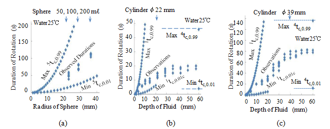
Figure 11: (a) The observed durations of fluid rotation in spherical flasks with volumes of 50, 100, and 200 mL are plotted as dots. The maximally and minimally expected durations of 5_t_c,0.99 and 5_t_c,0.01, which are proportional to r_2, are plotted as the upper and lower parabolic curves, respectively. (b), (c) The observed durations of fluid rotation in graduated cylinders with volumes of (b) 50 and (c) 200 mL are plotted as dots. For the case where the depth is less than the diameter of the cylinder (_h ≤ 2_a_), the maximally and minimally expected durations of 1_t_c,0.99 and 1_t_c,0.01, which are proportional to h_2, are plotted as the upper and lower parabolic curves, respectively. For the case where the depth is greater than the diameter of the cylinder (_h > 2_a_), the maximally and minimally expected durations of 4_t_c,0.99 and 4_t_c,0.01are plotted as the upper and lower straight lines, respectively. The observed durations are bounded by the two parabolic curves and two straight lines.