Multidimensional Interactive Cosmological Model: Chronological Evolution of Universe
Cosmological studies incorporate a set of differential equations which can be shown as an autonomous system. In our article, interactions are chosen. Solution of the dynamical system is analysed. Chevallier- Polarski-Linder dark energy model is opted and the concerned stability is studied. Point of periodicity is found to grow at high redshift for low dimensionless density parameters of matter. As we chronologically proceed towards the present time, this point is shifted towards high values of dimensionless density due to matter. At present time even the point of periodicity is seen to sustain. Distinguishably no attractor or past time attractor is noticed to get formed.
Mathematical Construction
We assume our universe to be filled up of baryonic matter, radiation and dark energy. The energy density is comprised of three distinct parts and the field equation looks like
$$H^2 = \frac{k}{3} \left( \rho_m + \rho_r + \rho_d \right)$$
(2)
Along with this, the equations of continuity for matter, radiation and dark energy turn to be
$$\dot{\rho}_m + 3H \rho_m = 0 \text{ (as } \rho_m = 0 \text{)}$$
(3)
$$\dot{\rho}_r + 4H \rho_r = 0 \text{ (as } \rho_r = \frac{1}{3} \rho_r \text{) and}$$
(4)
$$\dot{\rho}_d + 3H \rho_d \left\{ \left( 1 + \omega_0 \right) + \frac{\omega_r z}{1 + z} \right\} = 0$$
(5)
We derive an analogous equation with dimensionless density parameters as,
$$1 = \Omega_m + \Omega_z + \Omega_d$$
Where $\Omega_m = \frac{k \rho_m}{3H^2}$, $\Omega_z = \frac{k \rho_r}{3H^2}$ and $\Omega_d = \frac{k \rho_d}{3H^2}$ (6)
Differentiating the above first two expressions with respect to $N = \ln a(t)$, a(t) being the scale factor, we are led to derive the dynamical system as
$$\frac{d\Omega_m}{dN} = \Omega_m \left[ 3 \left( \Omega_m - 1 \right) + 4 \rho_r + 3 \left( 1 - \Omega_m - \Omega_r \right) \left\{ \left( 1 + \omega_0 \right) + \frac{\omega_r z}{1 + z} \right\} \right]$$
(7)
and
$$\frac{d\Omega_r}{dN} = \Omega_r \left[ 4 \left( \Omega_r - 1 \right) + 4 \rho_m + 3 \left( 1 - \Omega_m - \Omega_r \right) \left\{ \left( 1 + \omega_0 \right) + \frac{\omega_r z}{1 + z} \right\} \right]$$
(8)
Same kind of system is studied in the reference [8]. This reference has established that all the systems’ equilibrium points are such as $\Omega_m$ or/and $\Omega_r$ do/does vanish. Hence non-coupled matter, radiation and dark energy cannot produce a homoclinic orbit which needs a center equilibrium point with $\Omega_r \neq 0$.
This does not support a ΛCDM cosmology. The same is found to be true for any extended theories of gravity with an effective dark energy [9]. For instance an f(R) theory in Palatini formalism can be written in the reference [10] as
$$\Omega_m = k \frac{k \rho_m}{3F \xi H^2}, \Omega_r = k \frac{k \rho_r}{3F \xi H^2} \text{ and } \Omega_f = \frac{FR - f}{6F \xi H^2}$$
(9)
where $R$ is the usual scalar curvature, $F = \frac{df}{dR}$ and
$$\xi = \left[ 1 - \frac{3}{2} \frac{dF}{dR} \left( FR - 2f \right) / F \left( \frac{dF}{dR} - F \right) \right]^2$$
With the help of these, we can rewrite the dynamical equations as
$$\frac{d\Omega_m}{dN} = \Omega \left[ -3 + 3\Omega_m + 4\Omega_r + \left( 1 - \Omega_m - \Omega_r \right) C(R) \right]$$
(10)
and
$$\frac{d\Omega_r}{dN} = \Omega \left[ -4 + 3\Omega_m + 4\Omega_r + \left( 1 - \Omega_m - \Omega_r \right) C(R) \right]$$
(11)
$$C(R) = -3 \frac{\left( FR - 2f \right) \frac{dF}{dR} R}{FR - f \left( R \frac{dF}{dR} - F \right)}$$
Considering $C(R) = 3 \left\{ \left( 1 + \omega_0 \right) + \frac{\omega_r z}{1 + z} \right\}$, we can construct the same dynamical system.
Interactive System
In this model, we consider a dark energy coupled to both radiation and matter with coupling functions $Q_m$ and $Q_r$ respectively. We construct
$$q_m \frac{k}{3} Q_m \text{ and } q_r \frac{k}{3} Q_r$$
(12)
Following the reference [11], we construct a dynamical system
$$\frac{d\Omega_m}{dN} = \Omega_m \left[ -3 + 3\Omega_m + 4\Omega_r + \left( 1 - \Omega_m - \Omega_r \right) \left\{ \left( 1 + \omega_0 \right) + \frac{\omega_r z}{1 + z} \right\} + q_m$$
(13)
and
$$\frac{d\Omega}{dN} = \Omega \left[ -4 + 3\Omega_m + 4\Omega_r + 3(1 - \Omega_m - \Omega_r) \left( (1 + \omega_0) + \frac{\omega_r}{1 + z} \right) \right] + q_r$$
Now, we have to choose some possible and suitable values for $\Omega_{m(eq)}$, $\Omega_{r(eq)}$, $\frac{dq_m}{d\Omega_m}$, $\frac{dq_r}{d\Omega_r}$ and $\frac{dq_r}{d\Omega_m}$ such that some coupling functions allow homoclinic orbits around the center equilibrium point $(\Omega_{m(eq)}, \Omega_{r(eq)})$. Next, we will consider the special cases $q_m = 0$ and $q_r = 0$.
$$q_m = 0$$
We will try to find the central equilibrium points given by $(\Omega_{m(eq)}, \Omega_{r(eq)}) \neq 0$ when $q_m = 0$, responsible for homoclinic orbits. Eigen values that have to be pure imaginary numbers take the form
$$2\lambda_r = \left[ 8\Omega \frac{d\omega(z)}{d\Omega} + 18\Omega \frac{d\omega(z)}{d\Omega} + \Omega \frac{d\omega(z)}{d\Omega} + \omega(z) \right] + 3\Omega_r \left[ 3\Omega \frac{d\omega(z)}{d\Omega} + 2\Omega \frac{d\omega(z)}{d\Omega} + 3\omega(z) \right] + 2\Omega_r \left[ 3\Omega \frac{d\omega(z)}{d\Omega} + 2\Omega \frac{d\omega(z)}{d\Omega} + 3\omega(z) \right] + 3\Omega_r \left[ 3\Omega \frac{d\omega(z)}{d\Omega} + 2\Omega \frac{d\omega(z)}{d\Omega} + 3\omega(z) \right] + 3\Omega_r \left[ 3\Omega \frac{d\omega(z)}{d\Omega} + 2\Omega \frac{d\omega(z)}{d\Omega} + 3\omega(z) \right] + 3\Omega_r \left[ 3\Omega \frac{d\omega(z)}{d\Omega} + 2\Omega \frac{d\omega(z)}{d\Omega} + 3\omega(z) \right] + 3\Omega_r \left[ 3\Omega \frac{d\omega(z)}{d\Omega} + 2\Omega \frac{d\omega(z)}{d\Omega} + 3\omega(z) \right] + 3\Omega_r \left[ 3\Omega \frac{d\omega(z)}{d\Omega} + 2\Omega \frac{d\omega(z)}{d\Omega} + 3\omega(z) \right] + 3\Omega_r \left[ 3\Omega \frac{d\omega(z)}{d\Omega} + 2\Omega \frac{d\omega(z)}{d\Omega} + 3\omega(z) \right] + 3\Omega_r \left[ 3\Omega \frac{d\omega(z)}{d\Omega} + 2\Omega \frac{d\omega(z)}{d\Omega} + 3\omega(z) \right] + 3\Omega_r \left[ 3\Omega \frac{d\omega(z)}{d\Omega} + 2\Omega \frac{d\omega(z)}{d\Omega} + 3\omega(z) \right] + 3\Omega_r \left[ 3\Omega \frac{d\omega(z)}{d\Omega} + 2\Omega \frac{d\omega(z)}{d\Omega} + 3\omega(z) \right] + 3\Omega_r \left[ 3\Omega \frac{d\omega(z)}{d\Omega} + 2\Omega \frac{d\omega(z)}{d\Omega} + 3\omega(z) \right] + 3\Omega_r \left[ 3\Omega \frac{d\omega(z)}{d\Omega} + 2\Omega \frac{d\omega(z)}{d\Omega} + 3\omega(z) \right] + 3\Omega_r \left[ 3\Omega \frac{d\omega(z)}{d\Omega} + 2\Omega \frac{d\omega(z)}{d\Omega} + 3\omega(z) \right] + 3\Omega_r \left[ 3\Omega \frac{d\omega(z)}{d\Omega} + 2\Omega \frac{d\omega(z)}{d\Omega} + 3\omega(z) \right] + 3\Omega_r \left[ 3\Omega \frac{d\omega(z)}{d\Omega} + 2\Omega \frac{d\omega(z)}{d\Omega} + 3\omega(z) \right] + 3\Omega_r \left[ 3\Omega \frac{d\omega(z)}{d\Omega} + 2\Omega \frac{d\omega(z)}{d\Omega} + 3\omega(z) \right] + 3\Omega_r \left[ 3\Omega \frac{d\omega(z)}{d\Omega} + 2\Omega \frac{d\omega(z)}{d\Omega} + 3\omega(z) \right] + 3\Omega_r \left[ 3\Omega \frac{d\omega(z)}{d\Omega} + 2\Omega \frac{d\omega(z)}{d\Omega} + 3\omega(z) \right] + 3\Omega_r \left[ 3\Omega \frac{d\omega(z)}{d\Omega} + 2\Omega \frac{d\omega(z)}{d\Omega} + 3\omega(z) \right] + 3\Omega_r \left[ 3\Omega \frac{d\omega(z)}{d\Omega} + 2\Omega \frac{d\omega(z)}{d\Omega} + 3\omega(z) \right] + 3\Omega_r \left[ 3\Omega \frac{d\omega(z)}{d\Omega} + 2\Omega \frac{d\omega(z)}{d\Omega} + 3\omega(z) \right] + 3\Omega_r \left[ 3\Omega \frac{d\omega(z)}{d\Omega} + 2\Omega \frac{d\omega(z)}{d\Omega} + 3\omega(z) \right] + 3\Omega_r \left[ 3\Omega \frac{d\omega(z)}{d\Omega} + 2\Omega \frac{d\omega(z)}{d\Omega} + 3\omega(z) \right] + 3\Omega_r \left[ 3\Omega \frac{d\omega(z)}{d\Omega} + 2\Omega \frac{d\omega(z)}{d\Omega} + 3\omega(z) \right] + 3\Omega_r \left[ 3\Omega \frac{d\omega(z)}{d\Omega} + 2\Omega \frac{d\omega(z)}{d\Omega} + 3\omega(z) \right] + 3\Omega_r \left[ 3\Omega \frac{d\omega(z)}{d\Omega} + 2\Omega \frac{d\omega(z)}{d\Omega} + 3\omega(z) \right] + 3\Omega_r \left[ 3\Omega \frac{d\omega(z)}{d\Omega} + 2\Omega \frac{d\omega(z)}{d\Omega} + 3\omega(z) \right] + 3\Omega_r \left[ 3\Omega \frac{d\omega(z)}{d\Omega} + 2\Omega \frac{d\omega(z)}{d\Omega} + 3\omega(z) \right] + 3\Omega_r \left[ 3\Omega \frac{d\omega(z)}{d\Omega} + 2\Omega \frac{d\omega(z)}{d\Omega} + 3\omega(z) \right] + 3\Omega_r \left[ 3\Omega \frac{d\omega(z)}{d\Omega} + 2\Omega \frac{d\omega(z)}{d\Omega} + 3\omega(z) \right] + 3\Omega_r \left[ 3\Omega \frac{d\omega(z)}{d\Omega} + 2\Omega \frac{d\omega(z)}{d\Omega} + 3\omega(z) \right] + 3\Omega_r \left[ 3\Omega \frac{d\omega(z)}{d\Omega} + 2\Omega \frac{d\omega(z)}{d\Omega} + 3\omega(z) \right] + 3\Omega_r \left[ 3\Omega \frac{d\omega(z)}{d\Omega} + 2\Omega \frac{d\omega(z)}{d\Omega} + 3\omega(z) \right] + 3\Omega_r \left[ 3\Omega \frac{d\omega(z)}{d\Omega} + 2\Omega \frac{d\omega(z)}{d\Omega} + 3\omega(z) \right] + 3\Omega_r \left[ 3\Omega \frac{d\omega(z)}{d\Omega} + 2\Omega \frac{d\omega(z)}{d\Omega} + 3\omega(z) \right] + 3\Omega_r \left[ 3\Omega \frac{d\omega(z)}{d\Omega} + 2\Omega \frac{d\omega(z)}{d
Center equilibrium point can be written as
$$\left( \Omega_{m(eq)} , \Omega_{r(eq)} \right) = \left( -q_m , \frac{(z+1)q_m}{(3\omega_0 - 1)(z+1)} + 3\omega_1 z + q_m + 1 \right)$$
where $\Omega_{m(eq)} > 0, \Omega_{r(eq)} > 0$ and $\Omega_{m(eq)} + \Omega_{r(eq)} < 1$ if
$$q_m < \left( 3\omega_0 - 1 \right) + \frac{3\omega_1 z}{z+1}$$
The Eigen values $\lambda_z$ will be purely imaginary numbers if
$$\frac{dq_m}{d\Omega_m} = \left[ 3 \frac{d\omega(z)}{d\Omega_m} q_m \left( 3(q_m + 1) \left( \omega_0 + \frac{\omega_z}{z+1} \right) - 1 \right) + \left( 3\omega_0 + \frac{3\omega_z}{z+1} - 1 \right) \left( -3 \frac{d\omega(z)}{d\Omega_m} q_m + 9 \left( \omega_0 + \frac{\omega_z}{z+1} \right) - 9 \left( \omega_0 + \frac{\omega_z}{z+1} \right) \right] \left[ 1 - 3 \left( \omega_0 + \frac{\omega_z}{z+1} \right) \right]^2$$
and
$$\frac{dq_m}{d\Omega_m} < \left( \text{or} > \right) \left[ 3 \frac{d\omega(z)}{d\Omega_m} q_m + \left( 1 - 3 \left( \omega_0 + \frac{\omega_z}{z+1} \right) \right) ^2 - 3 \frac{d\omega(z)}{d\Omega_m} q_m + 3 \frac{d\omega(z)}{d\Omega_m} q_m \left( 3(q_m + 1) \left( \omega_0 + \frac{\omega_z}{z+1} \right) - 1 \right) \right] \left[ 3 \left( 1 - 3 \left( \omega_0 + \frac{\omega_z}{z+1} \right) \right) ^2 \left( \frac{d\omega(z)}{d\Omega_m} q_m + \left( \omega_0 + \frac{\omega_z}{z+1} \right) \right) \left( 3 \omega_0 + \frac{3\omega_z}{z+1} - 1 \right) \right]^1$$
when $q_m \frac{d\omega(z)}{d\Omega_m} > \left( \text{or} < \right) \left( \omega_0 + \frac{\omega_z}{z+1} \right) \left( 1 - 3 \left( \omega_0 + \frac{\omega_z}{z+1} \right) \right)$ for
$$\left( \Omega_{m(eq)}, \Omega_{r(eq)} \right).$$
Phase Space with CPL Parametrization
For the CPL parametrization $\omega(z) = \left( \omega_0 + \omega_1 \frac{z}{1+z} \right) [12]$, the best fit values of $\omega_0$ and $\omega_1$ with some data analysis, are $\omega_0 = -0.97$ and $\omega_1 = -0.57$ [13]. We have picked these values among tons of data analysis as we wanted such values of $\omega_0$ and $\omega_1$ which can signify the present time situation (phantom barrier), even when we do not consider the redshift. We have constructed a model inspired by the article [8], $\omega_0 = -0.97$ and $\omega_1 = -0.57$,
$$q_m = 0$$
$$q_r = \alpha \Omega_2 \omega_z$$
where $\alpha$ is a positive constant. Now, we are going to show the validity of stability of this model, using the equilibrium points we have got in the previous subsections.
Model Stability
We have equilibrium points for $\left( \Omega_{m(eq)} \Omega_{r(eq)} \right) \neq 0$, with the help of previous subsections as
$$\left( \Omega_{m(eq)} \Omega_{r(eq)} \right) = \left( 1 - \alpha \Omega_2 \left( 1 - \Omega_r - \Omega_m \right) \left( \frac{1+z}{2.91z + 4.62} + 1 \right), \alpha \Omega_2 \left( 1 - \Omega_r - \Omega_m \right) \right)$$
Corresponding eigen values are
$$2\lambda_z = \pm 1.71 \left[ -2\Omega_r^2 \left( -\Omega_r^2 \frac{d\omega}{d\Omega_r} \left( \Omega_r^2 \left( z(5.99 - 1.17\alpha) - 1.17\alpha - 2 \frac{d\omega}{d\Omega_r} + 3.99 \right) + 0.59\alpha - 0.59\alpha \Omega_m^2 \right) + 0.59\alpha - 0.59\alpha \Omega_m^2 \right] + 0.59\alpha - 0.59\alpha \Omega_m^2 \right] + 0.59\alpha - 0.59\alpha \Omega_m^2 \right] + 0.59\alpha - 0.59\alpha \Omega_m^2 \right] + 0.59\alpha - 0.59\alpha \Omega_m^2 \right] + 0.59\alpha - 0.59\alpha \Omega_m^2 \right] + 0.59\alpha - 0.59\alpha \Omega_m^2 \right] + 0.59\alpha - 0.59\alpha \Omega_m^2 \right] + 0.59\alpha - 0.59\alpha \Omega_m^2 \right] + 0.59\alpha - 0.59\alpha \Omega_m^2 \right] + 0.59\alpha - 0.59\alpha \Omega_m^2 \right] + 0.59\alpha - 0.59\alpha \Omega_m^2 \right] + 0.59\alpha - 0.59\alpha \Omega_m^2 \right] + 0.59\alpha - 0.59\alpha \Omega_m^2 \right] + 0.59\alpha - 0.59\alpha \Omega_m^2 \right] + 0.59\alpha - 0.59\alpha \Omega_m^2 \right] + 0.59\alpha - 0.59\alpha \Omega_m^2 \right] + 0.59\alpha - 0.59\alpha \Omega_m^2 \right] + 0.59\alpha - 0.59\alpha \Omega_m^2 \right] + 0.59\alpha - 0.59\alpha \Omega_m^2 \right] + 0.59\alpha - 0.59\alpha \Omega_m^2 \right] + 0.59\alpha - 0.59\alpha \Omega_m^2 \right] + 0.59\alpha - 0.59\alpha \Omega_m^2 \right] + 0.59\alpha - 0.59\alpha \Omega_m^2 \right] + 0.59\alpha - 0.59\alpha \Omega_m^2 \right] + 0.59\alpha - 0.59\alpha \Omega_m^2 \right] + 0.59\alpha - 0.59\alpha \Omega_m^2 \right] + 0.59\alpha - 0.59\alpha \Omega_m^2 \right] + 0.59\alpha - 0.59\alpha \Omega_m^2 \right] + 0.59\alpha - 0.59\alpha \Omega_m^2 \right] + 0.59\alpha - 0.59\alpha \Omega_m^2 \right] + 0.59\alpha - 0.59\alpha \Omega_m^2 \right] + 0.59\alpha - 0.59\alpha \Omega_m^2 \right] + 0.59\alpha - 0.59\alpha \Omega_m^2 \right] + 0.59\alpha - 0.59\alpha \Omega_m^2 \right] + 0.59\alpha - 0.59\alpha \Omega_m^2 \right] + 0.59\alpha - 0.59\alpha \Omega_m^2 \right] + 0.59\alpha - 0.59\alpha \Omega_m^2 \right] + 0.59\alpha - 0.59\alpha \Omega_m^2 \right] + 0.59\alpha - 0.59\alpha \Omega_m^2 \right] + 0.59\alpha - 0.59\alpha \Omega_m^2 \right] + 0.59\alpha - 0.59\alpha \Omega_m^2 \right] + 0.59\alpha - 0.59\alpha \Omega_m^2 \right] + 0.59\alpha - 0.59\alpha \Omega_m^2 \right] + 0.59\alpha - 0.59\alpha \Omega_m^2 \
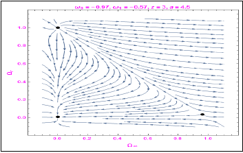
$$ \alpha = 4. 5 \mathrm {a n d} z = 3. $$
We have drawn a phase portrait (Figure 1), when α = 4.5 and z = 3. We can easily observe that actually it contains three points- two repeler points and one attractor i.e., two unstable points and one stable point.
First, let’s talk about the rappeler points. We have the first repellent at
$$ \Omega_ {r} \approx 1, \Omega_ {m} \approx 0. $$
. Clearly this point explains
the inflation stage of the universe as well as the radiation
dominated era i.e., the stage of the universe right after the Big
Bang when there is only radiation and no existence of dark
matter, dark energy. At this stage, the only cause of expansion
of the universe is radiation. We can observe from the above
phase portrait that every contour line is gone away from
this point implies, this unstable point signifies an unstable
universe and after that universe evolves. Again we have a second rappeler point at
$$ \mathrm {t} \Omega_ {m} \approx 1, \Omega_ {r} \approx 0. $$
. This signifies the
universe is completely dominated by dark matter. This point also signifies the unstable universe and after that universe evolves. Now, let’s talk about the attractor point.
We have got this point at 1 d Ω≈ i.e, the universe is fully dominated by dark energy. This attractor as well as stable point signify a stable universe. Now, we have constructed the whole dynamical system after considering the CPL parametrization of dark energy and we have taken the coupled function qr in our system. This coupled function qr represents the interaction between radiation and dark energy. After all these facts, we have an attractor which signifies such an incident. These kind of phase portraits are almost independent of redshift z i.e., during the plots of these phase portraits we have always the same three points at almost the same location for low and high redshifts. So we can conclude that if this kind of interaction between radiation and dark energy has taken place, our dynamical system does not support the future deceleration of the universe. Again since we have got the full dominance of the universe by dark energy- this rises to the fact that in the future the universe will undergo the cosmological singularity phenomena Big Rip. Now, we have considered the value of
$$ \omega_ {0} = - 0. 9 7 $$ $$ , \omega_ {1} = - 0. 5 7 $$
for our dark energy parametrization and if we
will consider the present time redshift z(=0) of the universe
then we can also mention the date of this Big Rip w.r.t present
time. The famous physicist Robert R. Caldwell gave a general
Big Rip scenario. According to this scenario for our model
there will be a Big Rip after 38 billion years from now.
Surprisingly we have identified some different behaviour of phase portraits when α > 5.4. These types of phase spaces are not independent of redshift z. These phase spaces are analysed below.
| Figure: 2.1 | Figure: 2.2 |
|---|---|
| Figure: 2.3 | Figure: 2.4 |
| Figure: 2.5 | Figure: 2.6 |
| Figure: 2.7 | Figure: 2.8 |
green contour line is appeared for each of the seven phase spaces. This green circular contour line represents the point of periodicity of our coupled model. We have noticed this point of periodicity moves downwards when the redshift z decreases from 4 to 0.01. This phenomena can be explained by the fact that when we consider the past accelerated situation of the universe to present time acceleration of the universe, value of the density parameter of dark matter will remain structured as we did not take any interaction of dark matter and dark energy i.e. qm = 0. Again, since we have assumed the interaction between radiation and dark energy, there is an abnormal variation in the values in Ωr. Since we have taken the coupled function $q_c = \alpha \Omega \Omega_d$, the interaction between radiation and dark energy become stronger. So, when we will defer redshift from $z = 4$ to $z = 0.01$ i.e., from past time situation of the universe to present era of the universe, we will get more accurate value of $\Omega$ but value of $\Omega_d$ defers. At redshift $z = 0.01$, we have $\Omega_d = -0.26$. Now, due to the high value of $\alpha$ the interaction has taken place between radiation and dark energy, becoming very high. For this purpose we have got some abnormal values of $\Omega_d$.
References
-
Wiggins S (2003) Introduction to applied nonlinear dynamical systems and chaos. Texts in Applied Mathematics 2: 844.
-
Deogharia G, Bandyopadhyay M, Biswas R (2020) Generalized model of interacting dark energy and dark matter: Phase portrait analysis of evolving universe. Modern Physics Letters A 36(40): 2150275.
-
Bahamonde S, Bohmer CG, Carloni S, Copeland EJ, Fang W, et al. (2018) Dynamical systems applied to cosmology: Dark energy and modified gravity. Physics Reports 775-777: 1-122.
-
Chaubey R, Raushan R (2016) Dynamical analysis of anisotropic cosmological model with quintessence. Astro-physics and Space Science 361: 06.
-
Aluri PK, Panda S, Sharma M, Thakur S (2013) Anisotropic universe with anisotropic sources. Journal of Cosmology and Astroparticle Physics 2013: 003.
-
Perez J, Fuzfa A, Carletti T, Melot L, Guedezounme L (2014) The jungle universe: coupled cosmological models in a lotka–volterra framework. General Relativity and Gravitation 46: 26.
-
Linder EV (2007) The dynamics of quintessence, the quintessence of dynamics. General Relativity and Gravitation 40: 329-356.
-
Fay S (2020) Acdm periodic cosmology. Monthly Notices of the Royal Astronomical Society 494(2): 2183-2190.
-
Capozziello S, De Laurentis M (2011) Extended theories of gravity. Physics Reports 509(4-5): 167-321.
-
Fay S, Tavakol R, Tsujikawa S (2007) ($R$) gravity theories in palatini formalism: Cosmological dynamics and observational constraints. Physical Review D 75: 063509.
-
Fay S (2014) From inflation to late time acceleration with a decaying vacuum coupled to radiation or matter. Phys Rev D 89: 063514.
-
Chevallier M, Polarski D (2001) Accelerating universes with scaling dark matter. International Journal of Modern Physics D 10(2): 213-223.
-
Gong Y, Gao Q, Zhu ZH (2013) The effect of different observational data on the constraints of cosmological parameters. Monthly Notices of the Royal Astronomical Society 430(4): 3142-3154.
- Asymmetry Irreversible Heterogeneity Quantum Cosmology Grand Mathematical PHYSICS
- Early Universe: Hadronic Crystals Coherent Micro Gravitational Wave Emitters PHYSICS Part II
- The Solar System Constraint Maze: A Scientific Dead-End Revealing the Interuniversal Machine
- Assessment of Radiofrequency Radiation from 2G and 3G Mobile Phone Handsets
- Early Universe Magneto-Gravitational Coupling Genesis Physics: Part I
- Falsifiability of the Classical Law of Gravitation and Unveiling the Time-temperature Entanglement of the Universe