Parameter Sensitivity of the Modified Green-Ampt Surface Sealing Infiltration Model
The Modified Green-Ampt Surface Sealing (MGASS) infiltration model considers real field infiltration process, wherein dispersed soil sediments, especially clay particles are present in the infiltrating water, and also accounts for the processof surface sealing. In view of the changes in the concentration of the soil sediments as infiltration proceeds, the various physical parameters in the equation are likely to change. Ponded infiltration studies were conducted in the field on three different soils to examine these changes in the model parameters, and how they influence the infiltration process. The results were compared with simulated infiltration using the Green-Ampt (G-A) MGASS infiltration models. The G-A model is often used to characterize infiltration process in soil hydrology. The key parameters in the MGASS model were the saturated hydraulic conductivity of the surface seal formed during the infiltration of water, hydraulic head, and moisture deficit; for the G-A model, the parameters were the saturated hydraulic conductivity of the soil surface, hydraulic head and moisture deficit. The saturated hydraulic conductivity (Ks) of the soil surface was found to be the most sensitive parameter in the G-A model. The MGASS equation, on the other hand was highly sensitive to changes in hydraulic head (hf).
Introduction
The Green-Ampt (G-A) model is a widely used physically-based hydrological model due to its acceptable physical origin and computational simplicity [1, 2, 3, 4]. The model assumes piston-type flow of soil water, and a step- function for soil water content within the profile. There are two distinct soil water contents in this situation, the initial water content θi and the saturated water content θs near the soil surface [5]. The cumulative infiltration amount can be calculated by iteration process as presented in Equation (1):
( ) ( ( )) ( )
Where, F is the cumulative infiltration amount [L]; Ks is the saturated hydraulic conductivity [L/T]; t is the time from the start of the infiltration [T]; ht is the pressure head [L]; is θs-θi the moisture deficit θd [L3/L3]; θi and θs are the initial and saturated moisture contents [L3/L3]
Since the development of the G-A model, it has gone through several series of modifications for various field conditions. For example, Mein and Larson [6] extended the model from ponded conditions to constant intensity conditions. Chu also applied this model to unsteady rainfall intensities. However, one major concern with regard to the applicability of the G-A model is the reason that infiltrating water always moves along with suspended soil sediments [7, 8], hence, the introduction of the Modified Green-Ampt Surface Sealing (MGASS) infiltration model (Equation 2).
( ) ( ) ( ( )) ( )
( ) ( ) where, F is the cumulative infiltration amount [L]; D is the mean particle diameter [L] of suspended sediments; d* is the dimensionless particle diameter of suspended sediments; Kx is the saturated hydraulic conductivity of the surface seal [L/T]; is the time from the start of the infiltration [T]; hf is the pressure head [L]; θs-θ_i is the moisture deficit θ_d[L3/L3]; θi and θs are the initial and saturated moisture contents [L3/L3]
The MGASS equation also incorporates the process of surface sealing and is capable of estimating the thickness of the surface seal formed as a result of the deposition of the suspended soil sediments, which is otherwise, difficult or almost impossible to measure experimentally [9]. Thus, the presence the soil particle phase in infiltrating water could greatly affect the infiltration process in the field. Additionally, just like all simulation models, prediction uncertainties arising from factors such as violation of underlying assumptions on which the model was developed, uncertainty in model parameters [10], and sensitivity of model parameters to changes are also expected in the field application of the MGASS equation.
Detailed reviews on the historic development of infiltration theory including the classic solutions based on the Richards’ equation have been provided [11]. This equation for soil moisture movement plays a very important role in contemporary engineering science, applied hydrology [12], soil science and agronomy. During model simulations, it is always imperative to estimate and report intrinsic prediction uncertainties, which usually result from the violation of assumptions inherent in the model, and also uncertainty in the model parameters [10]. However, it is very important to consider the fundamental assumptions on which these models are formulated since the unselective applications of theories developed for humid hydrology do not always carry out accurately in arid environments due to slaking of soil aggregates and dispersion of clays [9, 13]. No single model best meets all possible requirements, hence, in depth knowledge and understanding of model performance under different conditions are always required before valuable decisions and recommendations on the application of a model can be made. The choice of a model, would therefore, depend on the type of application, expected level of physical/mathematical rigour, and user preference [10].
Significant attempts have, thus, been made towards the quantification and reduction of prediction errors in infiltration models, however, most of these studies are characterized by limited assessment of model structure. Sensitivity analysis could serve as additional tool showing the relationship between model input factors and output variables in hydrologic modeling processes. This extensive analysis is key to identifying potential deficiencies in model structures and formulation, explain and correct the lack of fit of hydrological models, provide guidance for model reduction and parametrization, analyze the information content of available observations, and describe the subspace of the original control space driving predictive uncertainty [14]. Hence, the objective of the present study was to evaluate the parameter sensitivity of the MGASS model in comparison with the G- A model, and to determine their optimal parameters that would improve the utility of the models for simulating infiltration.
Materials and Methods
Field Infiltration Measurements
Field infiltration studies were conducted on three different soils, namely, Stagni-Dystric Gleysol (SDG), Plinthi Ferric Acrisol (PFA) and Plinthic Acrisol (PA). Ponded infiltration measurements were conducted using a single ring infiltrometer of 30 cm diameter and 20 cm height [9, 15]. The process involved inserting infiltrometer rings vertically into the soil to a depth of 10 cm with the aid of a mallet and a plank. Water at a pressure head of 5 cm was gently added in the extended cylinder, and maintained with water from a 1000 ml measuring cylinder. Infiltration was measured for 60 minutes. Initial measurements were conducted at regular time intervals of 30 seconds for five minutes after ponding when infiltration was very fast for the determination of sorptivity. The time interval was increased to 1, 3 and 5 minutes as infiltration slowed down towards the steady state. Analyses of infiltration parameters were done as discussed in Tuffour et al. [9].
Measurement of Saturated Hydraulic Conductivity
Saturated hydraulic conductivity was conducted on undisturbed soil cores in the laboratory using the modified falling head permeameter as described by Tuffour [13], and Bonsu and Laryea [16]. Intact soil cores were saturated for 24 hours; after which they were placed on gravels supported by a plastic sieve, and placed in a sink. Water was gently added to give hydraulic head in the extended cylinder and the fall of the hydraulic head (ht) on the soil surface was measured as a function of time (t) using a water manometer with a 5-meter scale. The Ks was estimated by the standard falling head equation:
( ) ( ) ( )
where, is the surface area of the cylinder [L2]; is the surface area of the soil [L2]; ho is the Initial hydraulic head [L]; L is the length of the soil column [L]; is the hydraulic head after a given time t [L]. Rewriting equation (1), a regression of ( ) on t with slope = ( ) was obtained. Since a=A in this particular case, Ks was simply calculated as:
( )
Sensitivity Analysis
Condition Number
Parameter perturbation was employed to provide a measure of the sensitivity of each model parameter [17]. Each parameter was varied by ±25%, ±50, and ±75% of its mean value. The parameters considered herein were Ks, hf and θd for the G-A model (Equation 1), and hf, θd and Kx for the MGASS model (Equation 2). The sensitivity of the cumulative infiltration amount was evaluated with each of these estimates varied about its mean value while all other parameter values were held constant. The condition number ( ) was calculated at six specific times, i.e., 5, 10, 15, 30, 45 and 60 minutes for each case.
̅ ( ) Where, CNp is the condition number [dimensionless] for the parameter p;p is the mean measured value for the parameter p; n is the dependent variable; ⧍p is the change in the independent variable; ∆n is the change in the dependent variable. In the present study, represented the cumulative infiltration amount (F), and p, a specific parameter of each model.
Sensitivity Index
Sensitivity of model outputs to the changes in input parameters was described according to Lenhart et al. [18]. and Ravazzani et al. [19]. Sensitivity of the model output to changes in the input parameters was described by a dimensionless sensitivity index [18]. Mathematically, a variable y is dependent on a parameter x by a partial derivative, ∂y/∂x which is numerically approximated by a finite difference. Assume is the model output computed from an initial value xo of the parameter x, which is varied by ±⧍x yielding x1 = xo-⧍x and x2 = xo+⧍x, yielding corresponding y1 and y_2, respectively. The finite approximation of the partial derivative ∂_y/∂x becomes:
( ) The dimensionless index was obtained by normalization as follows:
( ) ( ) The sign (i.e., positive or negative) of the index describes the direction of reaction of the model (i.e., if an increase of the parameter results in an increase of the output variable and a decrease of the parameter to a decrease of the variable, or inversely). For this study, ⧍x was fixed at 25% irrespective of the range of variation of tested parameters. Accordingly, the sensitivity of the model output was ranked according to Lenhart et al. [18] as presented in Table 1.
| Class | Index | Sensitivity | ||||||
|---|---|---|---|---|---|---|---|---|
| I | 0.00 | | 0.05 | Small to negligible | ||||||
| II | 0.05 | | 0.2 | Medium | ||||||
| III | 0.2 | | 1.00 | High | ||||||
| IV | | | 1.00 | Very high |
Table 1: Sensitivity index classes
| | Dimensionless sensitivity index Table 1: Sensitivity index classes
Results and Discussion
Results of sensitivity analysis on cumulative infiltration amount predicted from G-A and MGASS equations are presented in Table 2. The results show that the G-A equation is very sensitive to Ks and moderately sensitive to θd and hf. The MGASS equation, on the other hand showed high sensitivity to Kx, and negligible sensitivity to θd and hf.
| G-A Equation | MGASS Equation | |||||||||||||||||||
|---|---|---|---|---|---|---|---|---|---|---|---|---|---|---|---|---|---|---|---|---|
| Parameter | ||||||||||||||||||||
| SDG | PFA | PA | SDG | PFA | PA | |||||||||||||||
| (cm3/cm3) | I | I | I | II | II | II | ||||||||||||||
| (cm) | I | I | I | III | III | III | ||||||||||||||
| (cm/min) | III | IV | IV | - | - | - | ||||||||||||||
| (cm/min) | - | - | - | I | I | I |
Table 2: Sensitivity index classes of infiltration with G-A and MGASS equations.
SDG = Stagni-Dystric Gleysol; PFA = Plinthi Ferric Acrisol; PA = Plinthic Acrisol; *Gray shades describe negative values Table 2: Sensitivity index classes of infiltration with G-A and MGASS equations.
model parameter to perturbation are given by their varied condition numbers in Tables 3a – b for the G-A and MGASS and models, respectively.
| SDG | PFA | PA | ||||||||||||||||||||||||
|---|---|---|---|---|---|---|---|---|---|---|---|---|---|---|---|---|---|---|---|---|---|---|---|---|---|---|
| ΔB (%) | ||||||||||||||||||||||||||
| -25 | 0.26 | 3.75 | 0.24 | 0.76 | 3.75 | 0.32 | 0.99 | 3.75 | 0.46 | |||||||||||||||||
| -50 | 0.18 | 2.50 | 0.29 | 0.51 | 2.50 | 0.36 | 0.66 | 2.50 | 0.47 | |||||||||||||||||
| -75 | 0.088 | 1.25 | 0.34 | 0.25 | 1.25 | 0.39 | 0.33 | 1.25 | 0.48 | |||||||||||||||||
| Base value | 0.35 | 5.00 | 0.19 | 1.02 | 5.00 | 0.30 | 0.32 | 5.00 | 0.45 | |||||||||||||||||
| +25 | 0.44 | 6.25 | 0.14 | 1.27 | 6.25 | 0.15 | 1.65 | 6.25 | 0.050 | |||||||||||||||||
| +50 | 0.53 | 7.50 | 0.088 | 1.53 | 7.50 | 0.18 | 1.97 | 7.50 | 0.061 | |||||||||||||||||
| +75 | 0.61 | 8.75 | 0.037 | 1.78 | 8.75 | 0.22 | 2.30 | 8.75 | 0.071 |
Table 3: Sensitivity of cumulative infiltration amount with G-A equation.
ΔB = Change in base parameter value; SDG = Stagni-Dystric Gleysol; PFA = Plinthi Ferric Acrisol; PA = Plinthic Acrisol Table 3a: Changes in base parameter value in Green & Ampt equation.
| SDG | PFA | PA | |||||||||||||||||||||||
|---|---|---|---|---|---|---|---|---|---|---|---|---|---|---|---|---|---|---|---|---|---|---|---|---|---|
| ΔB (%) | |||||||||||||||||||||||||
| -25 | 4.1E-4 | 3.75 | 0.24 | 9.8E-4 | 3.75 | 0.33 | 1.1E-3 | 3.75 | 0.46 | ||||||||||||||||
| -50 | 2.7E-4 | 2.50 | 0.29 | 6.5E-4 | 2.50 | 0.36 | 7.5E-4 | 2.50 | 0.47 | ||||||||||||||||
| -75 | 1.4E-4 | 1.25 | 0.34 | 3.3E-4 | 1.25 | 0.39 | 3.7E-4 | 1.25 | 0.48 | ||||||||||||||||
| Base value | 5.5E-5 | 5.00 | 0.19 | 1.3E-3 | 5.00 | 0.30 | 1.5E-3 | 5.00 | 0.45 | ||||||||||||||||
| +25 | 6.8E-4 | 6.25 | 0.14 | 1.6E-3 | 6.25 | 0.27 | 1.9E-3 | 6.25 | 0.050 | ||||||||||||||||
| +50 | 8.2E-4 | 7.50 | 0.088 | 2.0E-3 | 7.50 | 0.24 | 2.2E-3 | 7.50 | 0.061 | ||||||||||||||||
| +75 | 9.6E-4 | 8.75 | 0.037 | 2.3E-3 | 8.75 | 0.21 | 2.6E-3 | 8.75 | 0.071 |
Table 4: Sensitivity of cumulative infiltration amount with G-A equation.
ΔB = Change in base parameter value; SDG = Stagni-Dystric Gleysol; PFA = Plinthi Ferric Acrisol; PA = Plinthic Acrisol Table 3b: Changes in base parameter value in the MGASS equation.
Green-Ampt Model Sensitivity
Table 4 shows a summary of the sensitivity of G-A equation to F. Figures 1 – 3 show the trend of cumulative infiltration amount to changes in Ks, θd and hf. Cumulative infiltration amount was significantly sensitive to changes in the θd, hf, and the Ks in respect of the condition numbers (Table 3a) but less sensitive to changes in θd and hf.
| SDG | PFA | PA | |||||||||||||||||||||||||||
|---|---|---|---|---|---|---|---|---|---|---|---|---|---|---|---|---|---|---|---|---|---|---|---|---|---|---|---|---|---|
| ΔB (%) | |||||||||||||||||||||||||||||
| -25 | 18.06 | 22.93 | 23.67 | 50.54 | 46.94 | 46.14 | 66.03 | 84.53 | 85.88 | ||||||||||||||||||||
| -50 | 12.80 | 22.48 | 23.98 | 35.27 | 43.94 | 46.46 | 46.29 | 83.11 | 85.99 | ||||||||||||||||||||
| -75 | 7.53 | 21.92 | 24.26 | 19.99 | 42.77 | 46.77 | 26.55 | 81.42 | 86.09 | ||||||||||||||||||||
| Base value | 23.32 | 23.32 | 23.32 | 46.74 | 46.74 | 46.74 | 85.77 | 85.77 | 85.77 | ||||||||||||||||||||
| +25 | 28.58 | 23.65 | 22.91 | 81.08 | 46.80 | 45.46 | 105.51 | 86.88 | 85.67 | ||||||||||||||||||||
| +50 | 33.84 | 23.94 | 22.41 | 96.35 | 47.31 | 45.09 | 125.25 | 87.89 | 85.57 | ||||||||||||||||||||
| +75 | 39.10 | 24.21 | 21.78 | 111.62 | 47.97 | 44.71 | 144.99 | 88.82 | 85.46 |
Table 5: Sensitivity of cumulative infiltration amount with G-A equation.
ΔB = Change in base parameter value; SDG = Stagni-Dystric Gleysol; PFA = Plinthi Ferric Acrisol; PA = Plinthic Acrisol Table 4: Sensitivity of cumulative infiltration amount with G-A equation.
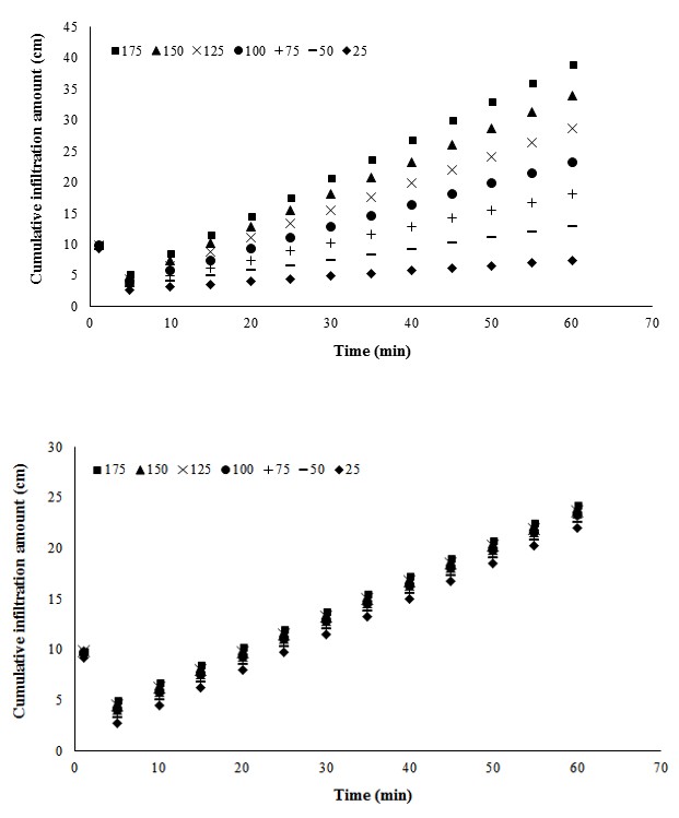
Figure 1a: Effects of changes in saturated hydraulic conductivity in the G-A model on cumulative infiltration amount in the Stagni-Dystric Gleysol.
Figure 1b: Effects of changes in pressure head in G-A model on cumulative infiltration amount in the Stagni-Dystric Gleysol.
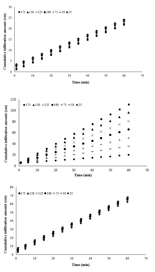
Figure 1c: Effects of changes in soil moisture content in the G-A model on cumulative infiltration amount in the Stagni-Dystric Gleysol.
Figure 2a: Effects of changes in saturated hydraulic conductivity in the G-A model on cumulative infiltration amount in the Plinthi Ferric Acrisol.
Figure 2b: Effects of changes in pressure head in the G-A model on cumulative infiltration amount in the Plinthi Ferric Acrisol.
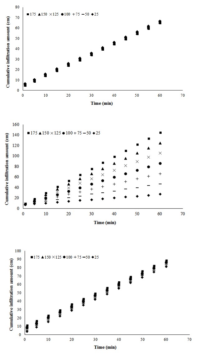
Figure 2c: Effects of changes in soil moisture content in the G-A model on cumulative infiltration amount in the Plinthi Ferric Acrisol.
Figure 3a: Effects of changes in saturated hydraulic conductivity in the G-A model on cumulative infiltration amount in the Plinthic Acrisol.
Figure 3b: Effects of changes in pressure head in the G-A model on cumulative infiltration amount in the Plinthic Acrisol.
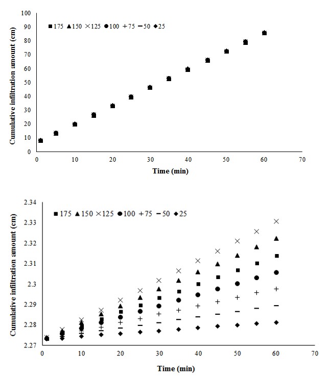
Figure 3c: Effects of changes in soil moisture content in the G-A model on cumulative infiltration amount in the Plinthic Acrisol.
MGASS Model Sensitivity
Table 5 shows a summary of the sensitivity of MGASS
equation to cumulative infiltration amount. Figures 4 – 6 show the responses of F to changes in Kx, hf and θd.
| SDG | PFA | PA | |||||||||||||||||||||||||||
|---|---|---|---|---|---|---|---|---|---|---|---|---|---|---|---|---|---|---|---|---|---|---|---|---|---|---|---|---|---|
| ΔB (%) | |||||||||||||||||||||||||||||
| -25 | 2.30 | 1.92 | 2.66 | 4.79 | 3.93 | 5.14 | 6.88 | 5.66 | 7.01 | ||||||||||||||||||||
| -50 | 2.29 | 1.47 | 2.97 | 4.77 | 2.94 | 5.46 | 6.86 | 4.25 | 7.12 | ||||||||||||||||||||
| -75 | 2.28 | 0.91 | 3.25 | 4.75 | 1.76 | 5.77 | 6.83 | 2.55 | 7.22 | ||||||||||||||||||||
| Base value | 2.31 | 2.31 | 2.31 | 4.81 | 4.81 | 4.81 | 6.90 | 6.90 | 6.90 | ||||||||||||||||||||
| +25 | 2.31 | 2.64 | 1.90 | 4.82 | 5.59 | 4.46 | 6.92 | 8.01 | 6.81 | ||||||||||||||||||||
| +50 | 2.32 | 2.93 | 1.40 | 4.84 | 6.31 | 4.09 | 6.95 | 9.02 | 6.70 | ||||||||||||||||||||
| +75 | 2.33 | 3.20 | 0.77 | 4.86 | 6.97 | 3.71 | 6.97 | 9.95 | 6.60 |
Table 6: Sensitivity of cumulative infiltration amount with MGASS equation.
ΔB = Change in base parameter value; SDG = Stagni-Dystric Gleysol; PFA = Plinthi Ferric Acrisol; PA = Plinthic Acrisol Table 5: Sensitivity of cumulative infiltration amount with MGASS equation.
Figure 4a: Effects of changes in surface seal saturated hydraulic conductivity in the MGASS model on cumulative infiltration amount in the Stagni-Dystric Gleysol.
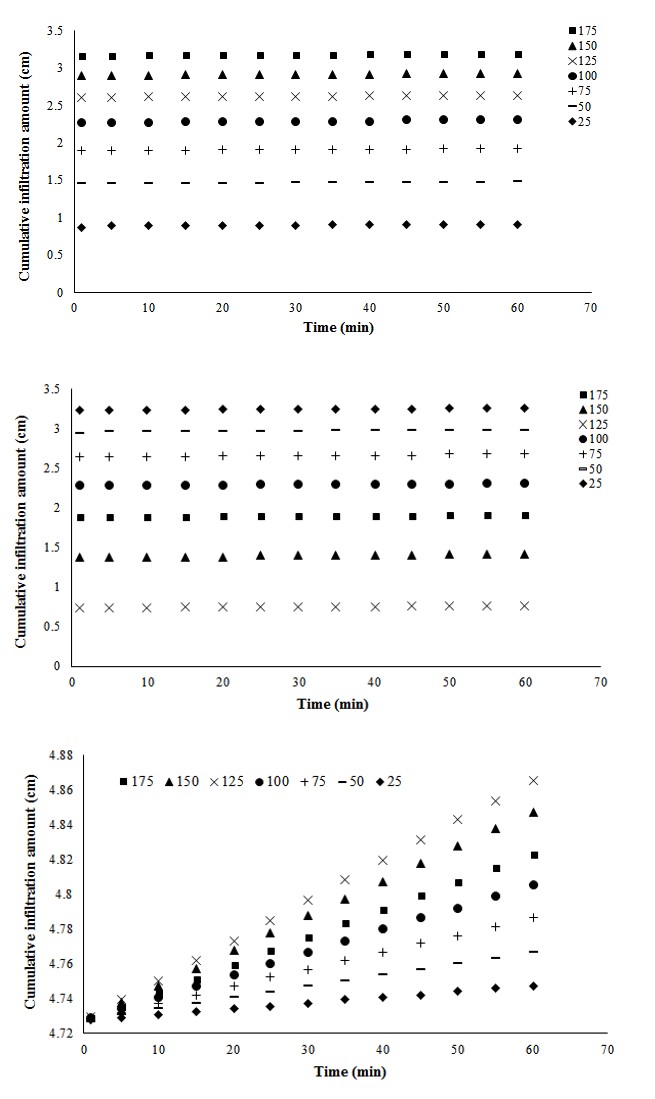
Figure 4b: Effects of changes in the pressure head in the MGASS model on cumulative infiltration amount in the Stagni-Dystric Gleysol.
Figure 4c: Effects of changes in the soil moisture content in the MGASS model on cumulative infiltration amount in the Stagni-Dystric Gleysol.
Figure 5a: Effects of changes in surface seal saturated hydraulic conductivity in the MGASS model on cumulative infiltration amount in the Plinthi Ferric Acrisol.
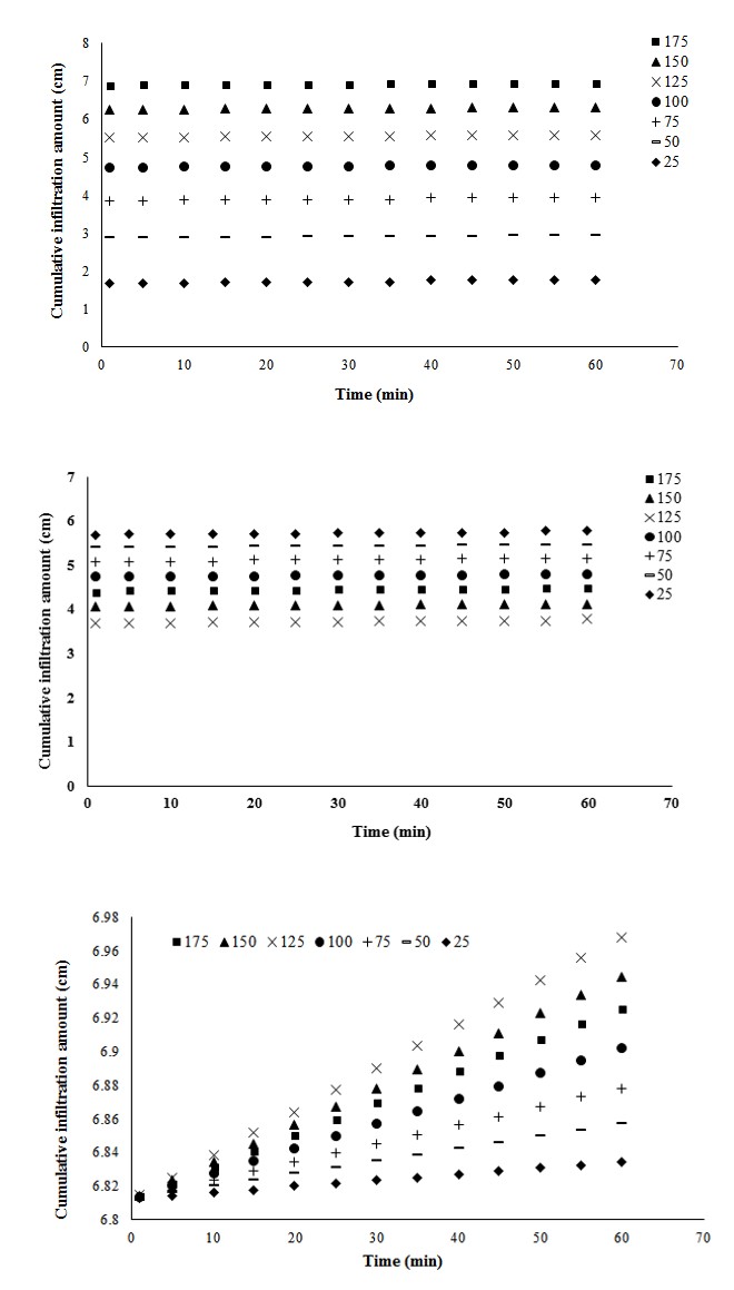
Figure 5b: Effects of changes in the pressure head in the MGASS model on cumulative infiltration amount in the Plinthi Ferric Acrisol.
Figure 5c: Effects of changes in the soil moisture content in the MGASS model on cumulative infiltration amount in the Plinthi Ferric Acrisol.
Figure 6a: Effects of changes in surface seal saturated hydraulic conductivity in the MGASS model on cumulative infiltration amount in the Plinthic Acrisol.
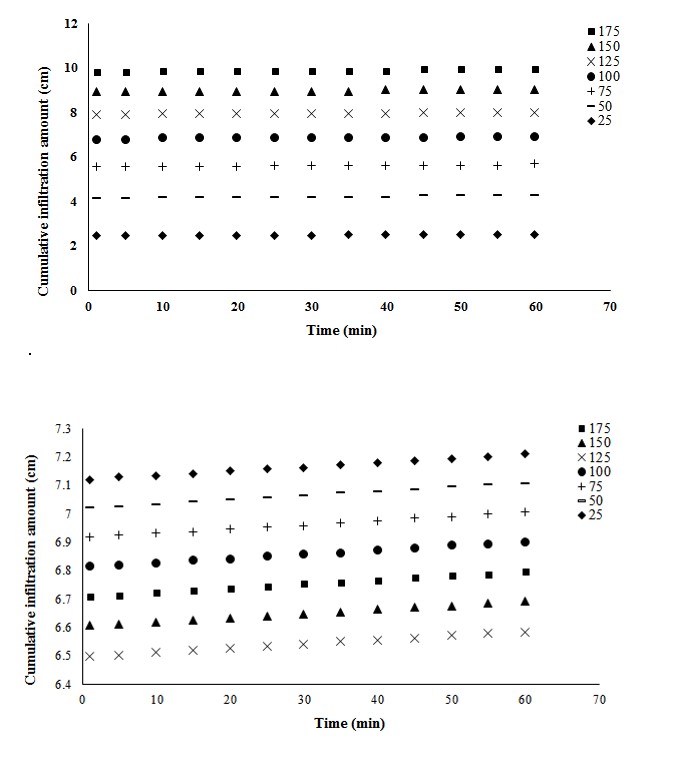
Figure 6b: Effects of changes in the pressure head in the MGASS model on cumulative infiltration amount in the Plinthic Acrisol.
Figure 6c: Effects of changes in the soil moisture content in the MGASS model on cumulative infiltration amount in the Plinthic Acrisol.
change in F. However, changes in F resulting from changes in hf were high (Table 2). Sensitive parameters show strong differences between the two models.
Altogether, sensitivity analysis was successful in identifying the most important parameter in both infiltration equations, although different results with regard to parameter sensitivities were obtained. Thus, insights on which parameter(s) contribute most to the outputs of the models have been achieved. Classification of parameters were different, which could on the most part have resulted from the differences of the sensitivity index around the class boundaries. Sensitivity analysis has proven to be a valuable tool for the assessment of the input parameters with respect to their impact on model output, and can thus, be very essential model validation and reduction of uncertainty [20].
Conclusion
A comparison of two infiltration equations has been presented in this study. Results showed that, the MGASS equation was highly sensitive to changes in hf followed by θd and Kx. The Green-Ampt equation, on the other hand responded extremely high to changes in the Ks than hf and θd, respectively. Thus, hydraulic head, moisture content, and saturated hydraulic conductivity of the soil surface were found to be the key parameters influencing infiltration of water in soils in the MGASS and G-A equations, respectively. Thus, the output of a particular model not only depends on the structure of the model, but also on the input parameters. The current study was successful in identifying the most important input parameter (i.e., _h_f) in the MGASS equation, which should be given key consideration during the calibration and validation of the MGASS equation.
References
-
Green WH, Ampt GA (1911) Studies on soil physics: I. Flow of air and water through soils. J Agric Sci 4: 1-24.
-
O’Brien JS, Jorgensen C, Garcia R (2009) FLO-2D Software. Version 2009, FLO-2D Software, Inc. Nutrioso, AZ, Nutrioso, AZ.
-
Rossman LA (2010) Storm Water Management Model User’s Manual, version 5.0. National Risk Management Research Laboratory, Office of Research and Development, US Environmental Protection Agency.
-
Arnold JG, Moriasi DN, Gassman PW, Abbaspour KC, White MJ, et al. (2012) SWAT: Model use, calibration, and validation. Trans ASABE 55(4): 1491-1508.
-
Chen L, Xiang L, Young MH, Yin J, Yu Z, et al. (2015) Optimal parameters for the Green-Ampt infiltration model under rainfall conditions. J Hydrol Hydromech 63(2): 93-101.
-
Mein RG, Larson CL (1973) Modeling infiltration during a steady rain. Water Res Res 9(2): 384-394.
-
Chu ST (1978) Infiltration during unsteady rain. Water Res Res 14(3): 461-466.
-
Tuffour HO, Bonsu M (2015) Application of Green and Ampt Equation to infiltration with soil particle phase. Int J Sci Res Agric Sci 2(4): 76-88.
-
Tuffour HO, Bonsu M, Quansah C, Abubakari A (2015) A physically-based model for estimation of surface seal thickness. Int J Ext Res 4: 60-64.
-
Clausnitzer V, Hopmans JW, Starr L (1998) Parameter uncertainty analysis of common infiltration models. Soil Sci Soc Am J 62(6): 1477-1487.
-
Youngs EG (1995) The physics of infiltration. Soil Sci Soc Am J 59(2): 307-313.
-
Islam MS (2017) Sensitivity analysis of unsaturated infiltration flow using head based finite element solution of Richards’ equation. Matematika 33(2): 131-148.
-
Tuffour HO (2015) Physically based modelling of water infiltration with soil particle phase. Ph.D. Dissertation, Kwame Nkrumah University of Science and Technology, Ghana.
-
Castaings W, Dartus D, LeDimet FX, Saulnier GM (2007) Sensitivity analysis and parameter estimation for the distributed modeling of infiltration excess overland flow. Hydrology and Earth System Sciences Discussions. Euro Geosci Union 4(1): 363-405.
-
Khalid AA, Tuffour HO, Bonsu M (2014) Influence of Poultry Manure and NPK Fertilizer on Hydraulic Properties of a Sandy Soil in Ghana. Int J Sci Res Agric Sci 1(2): 16-22.
-
Bonsu M, Laryea KB (1989) Scaling the saturated hydraulic conductivity of an Alfisol. J Soil Sci 40(4): 731-742.
-
Chapra SC (1997) Surface Water-quality Modeling. New York, NY, McGraw-Hill.
-
Lenhart T, Eckhardt K, Fohrer, N, Frede H-G (2002) Comparison of two different approaches of sensitivity analysis. Phys Chem Earth J 27: 645-654.
-
Ravazzani G, Caloiero T, Feki M, Pellicone G (2018) Impact of Infiltration Process Modeling on Runoff Simulations: The Bonis River Basin. Proceedings 2(11): 638.
-
Turner ER (2006) Comparison of infiltration equation and their field validation with rainfall simulation. MSc. Thesis, Department of Biological Resources Engineering, University of Maryland, USA.
- Enhancement of Vegetative Growth and Fruit Yield in Cucumber (Cucumis sativus L.) via Spiritual Blessing (Biofield) Energy Intervention
- Production of Açaí (Euterpe oleracea Mart.) under Different Agroforestry System Management Intensities in Amazonian Floodplain (Varzea) Forests
- Coffee and the Production Region: What is the Secret to the Expression "Quality"?
- Experiential Agripreneurship Training in Sub-Saharan Africa: Integrating a Business Incubator into Postgraduate Livestock Education at the University of Buea
- Advances in Agricultural High-Quality Development
- Linking Compost Residue to ABAGE in Plants - a Short Note