Gas Lift System
Generally, a gas lift is a flexible, and a reliable artificial lift system with the ability to cover a wide range of production rates. Gas lift systems are a closed system empowered by high- pressured gas. The entire process is used to reduce the wellbore fluid pressure gradient by supplementing gas through an external source to withdraw more liquid from the reservoir under higher drawdown. Many parameters affect a gas lift system design, such as changes in the wellhead and bottomhole pressures (BHPs), produced fluid type, and productivity index of the wellbore. As these parameters change, the gas injection pressure changes. Gas lift system demands a surface compressing unit and in the well gas lifts valves (GLVs). Overall, a gas lift system is a forgiving method of enhanced production, in other words, even a poor gas lift design may increase production. To achieve a higher ramp in fluid production rate using gas lift, however, a more sophisticated design of each compartment of the system is required.
History of Gas Lift
During its almost 150-year history, gas lift is considered as the most efficient artificial methods that may be effectively applied in the oilfields. The initial laboratory experiments using compressed air to lift liquids were conducted by Carl Loscher in Germany, 1797. This method was later used to lift water from pit swing. In this technique, air was injected into liquid at the bottom of tubing through a valve. Gas lift operation is a single point injection. It has been documented that in 1864 the same concept was applied in the oil industry, called a ‘well blower’ [1]. Cockford, an American engineer, used compressed air to lift produced oil from wells in Pennsylvania. According to Cloud, Cockford’s system consisted of an air-filled pipe connected to the tubing to decrease hydrostatic pressure by reducing oil density, allowing the well produce more [2]. Cockford’s technique continued to be used until 1920. Between 1920 and 1929, for safety reason, natural gas was tested to be used instead of compressed air. Due to successful test results, this method was then applied in the Seminole field- Oklahoma. Initially, gas was injected unrestrainedly into the bottom of the well. Due to low achievable injection pressures, gas lift application was limited to shallow wells. Downhole equipment used in the gas-lifted wells underwent a great evolution and early open installations utilizing a tubing string, were gradually replaced with installations including a packer and standing valve. Spring-operated differential GLV was invented in 1930s. This valve gets opened if the injected pressure (casing pressure) becomes greater than tubing pressure.
Running GLV and other downhole devices became easier and more cost effective by deploying wire line retrievable equipment in the 1930. Another GLVs model, which mechanically operated from the surface, was developed by Brown in1980 [3]. These valves are run in the well using tubing string, and if they need to be replaced, the whole tubing string has to be pulled out of the well. Due to the difficulty and unreliability of tubing retrievable GLVs, wire line retrievable GLVs were introduced. In the case of failure, wire line retrievable valves are replaced without pulling out the entire tubing string. Gas lift is not the best option for low production wells; therefore newer lifting methods such as chamber and plunger lift were introduced to produce from the wells with low liquid capacities.
Gas Lift System
Not all the oil wells start producing fluid naturally right after they put back online due to low Bottom Hole Pressure (BHP) which is insufficient to lift the fluid to the surface. At some point, the reservoir energy will not be sufficient to bring the reservoir fluid up to the surface because its energy is depleted. One way to help a well flow is to energize the reservoir fluid with a lighter fluid as the carrying fluid. In that case, the overall fluid density will drop which results in larger lift capability of the reservoir. Gas lift is the form of artificial lift that most closely resembles the natural flow process. It may be treated as the extension of the natural flow process. In a naturally flowing well, as the fluid travels upward toward the surface, the fluid column pressure is reduced causing the gas to expand and move faster upward. Injected gas will help carrying some diluted liquid to the surface; however, if the gas velocity is not high enough, some liquid may start to fall off at some point near surface. Gas lift is frequently used in lifting water for the purpose of gas deliquefication. In this approach, a high-pressure gas is injected into the fluid column to reduce the flowing pressure gradient. In other words; gas lift is the process of supplementing additional gas (from an external source) to increase the gas-liquid ratio (GLR) resulting in reducing the flowing fluid density. This process considered an expansion of natural flow phase. Figure 1 shows the schematic of a typical gas lift system. Compared to the other artificial lift methods, gas lift is simpler, more adaptable, and more efficient at wide ranges of fluid production There are two types of gas lift systems: continuous flow and intermittent flow. In both gas lift systems, high- pressure natural gas is injected from the surface to lift formation fluid. Continuous flow gas, which is very similar to the natural flow, is the most common gas lift method in the industry. In this technique, injecting gas into the production conduit at the maximum depth depending on the injection pressure and well depth results in an increase in the formation gas liquid ratio. Hence, both the density of the produced fluid and flowing pressure gradient of the mixture decrease which lead to a lower bottomhole pressure. Lower bottomhole pressure improves wellbore productivity index. Intermittent gas lift operation is achieved by injecting gas at sufficient volume and pressure into the tubing at the point below the fluid column to lift the liquid to the surface. Intermittent flow is periodic displacement of liquid from the tubing by injection high pressure gas into the wellbore. The advantage of intermittent flow gas lift over the continue gas lift is periodic need of high pressure gas. On the other hand, since gas is injected intermittently over specific period of time, this method is not capable of producing at high volume rate compared to continuous flow gas lift.
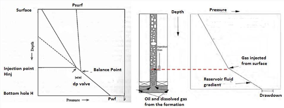
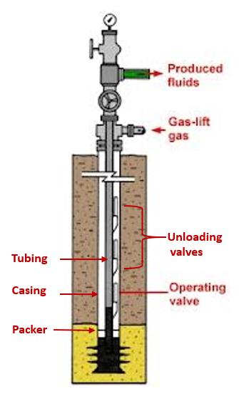
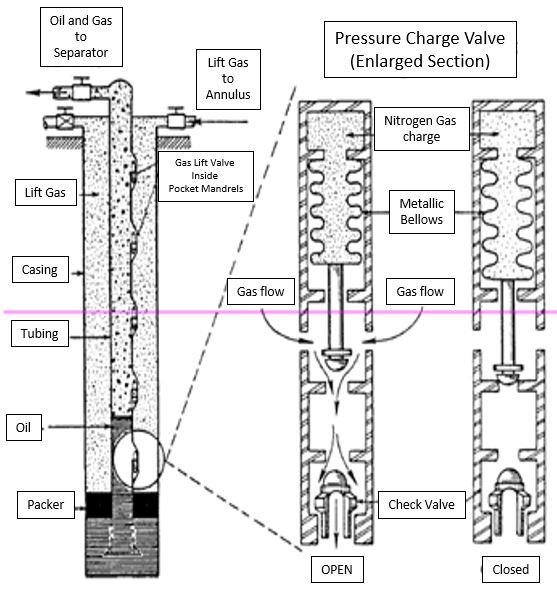
![Figure 1: Typical Gas Lifts System. Gas lift system is a closed system which requires a high pressure source of gas, surface controls, subsurface equipment, flow lines, separation and storage equipment, compressors, and GLVs. The effectiveness of a gas lift system depends on appropriate design of all these components. To achieve an efficient operation and to ensure that the suitable amount of gas is injected at all times, gas entry must be controlled by utilizing a downhole device. In modern practice, gas lift valves are used for downhole gas injection control. Because of its importance, various gas lift valves have been developed over the years. Gas lift system may be used to resume production from a well since the primary production ceases until its abandonment. Also, it may be used to increase the production from low producing wells. Initially, continuous gas lift may be used to produce at high liquid rates up to 50,000 STB/D [4]. Later, as both formation pressure and liquid rates gradually declined; replacing it with an intermittent gas lift system ensures that production goals are met. Gas lift system is the only form of artificial lift system that does not need downhole pump. However, this system is unable to significantly reduce BHP. The minimum required pressure gradient is approximately 0.22 psi/ft and rarely goes below 0.15 psi/ft as suggested by Pablano, & Fairuzov [5]. Therefore, gas lift system is a good candidate for projects where the BHP is constant. The higher production rate may be attained when the bottom GLV installed at the deepest point. Before starting gas injection, the required injection pressure has to be calculated based on the hydrostatic pressure inside the tubing at the depth where the valve will be installed. The location of first valve must be determined for kick- off. The high pressure gas in the annulus forces the liquid out of the tubing through U-tubing. Figure 2 demonstrates the point of injection.](/fulltextimages/989/fig_1.png)
Figure 1: Typical Gas Lifts System. Gas lift system is a closed system which requires a high pressure source of gas, surface controls, subsurface equipment, flow lines, separation and storage equipment, compressors, and GLVs. The effectiveness of a gas lift system depends on appropriate design of all these components. To achieve an efficient operation and to ensure that the suitable amount of gas is injected at all times, gas entry must be controlled by utilizing a downhole device. In modern practice, gas lift valves are used for downhole gas injection control. Because of its importance, various gas lift valves have been developed over the years. Gas lift system may be used to resume production from a well since the primary production ceases until its abandonment. Also, it may be used to increase the production from low producing wells. Initially, continuous gas lift may be used to produce at high liquid rates up to 50,000 STB/D [4]. Later, as both formation pressure and liquid rates gradually declined; replacing it with an intermittent gas lift system ensures that production goals are met. Gas lift system is the only form of artificial lift system that does not need downhole pump. However, this system is unable to significantly reduce BHP. The minimum required pressure gradient is approximately 0.22 psi/ft and rarely goes below 0.15 psi/ft as suggested by Pablano, & Fairuzov [5]. Therefore, gas lift system is a good candidate for projects where the BHP is constant. The higher production rate may be attained when the bottom GLV installed at the deepest point. Before starting gas injection, the required injection pressure has to be calculated based on the hydrostatic pressure inside the tubing at the depth where the valve will be installed. The location of first valve must be determined for kick- off. The high pressure gas in the annulus forces the liquid out of the tubing through U-tubing. Figure 2 demonstrates the point of injection.
Installing GLVs at deep depths is vitally important, and depends on the valve design, and its opening and closing pressures. The order of GLVs installation is of great importance in the lifting process. If the installation is not in the correct order, the gas lift system will fail. In a gas lift system design, the valves’ operating pressures drop as it gets deeper. Therefore, as the injection pressure drops, the upper valve operating at a higher injection pressure
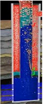
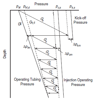
closes and lower valve starts to unload the well and so forth. Usually the lowest GLV is an open orifice plate, which is open all the time. In the Figure 4, the gas is injected from the casing and the reservoir fluid is produced through the tubing. Figure 5 demonstrates the valve depth determination with respect to the flowing tubing pressure.
Advantages of Gas Lift
In terms of production rate ranges and depth of lift, the gas lift system is flexible and can rarely be matched by other artificial lift methods if required injection gas pressure and volume are existed. Gas lift is one of the most flexible artificial lift techniques which even unappropriated design will still lift some fluid. Highly deviated wells with high formation GLR and sand production are good candidates for gas lift when artificial lift is needed.
Limitations of Gas Lift
Large well spacing for onshore wells and limited offshore platforms space for compressors may restrict the gas lift application. Gas lift is rarely applicable to single well installation and not appropriate for widely-spaced wells due to the difficulty of locating the power system centrally. Gas lift is not the option for viscous crude oil, super-saturated brine or emulsion fluid. In addition, the
Gas Lift Valve (GLV)
GLV is the heart of a gas lift system because of controlling production rates. The GLV is a backpressure regulator which functions based on the differential pressure between the injection gas pressure and the production fluid pressure [9]. The GLV regulates the pressure on its upstream side to its downstream. The architectural design of each GLV is as important as the depth of installation and number of GLVs used in each installation. Poor designs may result in installing dozens of GLVs to unload well that may not to be necessary.
Therefore, calibrating each GLV to achieve the best performance at the wellbore is vital to the artificial lift cycle of each well. Because a GLV consists of many movable mechanical compartments, achieving synergy between all those compartments should result in the best performance. The performance of a GLV affects both the technical and economic aspects of fluid lifting process. The main duty of a GLV is to allow the required amount of injected gas enter the wellbore to unload the well. If the designed parameters such as pressure column, water cut, GLR and well deliverability change, the GLVs may be installed at different depths to adjust the gas lift system accordingly. Figure 6 demonstrates the GLV at different depths.
![Figure 6: GLVs in vertical well. Before 1944 and prior to introducing bellows-charged GLVs, the most common GLV was the differential valve. The differential pressure between the injecting gas in the casing and the fluid inside the tubing controlled the operation of the valve. The differential valve, however, had some shortcomings in the unloading process and the differential valves had to be spaced closely together, little surface control was possible, and the valve was bulky and difficult to transport. Since then, better GLVs designs for better unloading of wells were developed. King patented the first GLV with single element, and charged bellows [10]. Today’s pressure operated gas lift valve has been modified little since King’s original valve. The King’s valve was designed to lift a low volume of liquid as it has a small chamber attached to its end section. The success of the King valve is the evidence that the basic principles used in the design were quickly adopted by almost all GLV manufacturers and are still used with little modification. Brown describes four types of GLVs: casing pressure operated valve, throttling valve, fluid operated valve, and combination valve [3]. The pressure operated valve is used in most gas lift installations. The gas lift valve has a loading element, which is a spring, a nitrogen charged bellows, or a combination of the two. The loading element provides the downward closing force in a gas lift valve.](/fulltextimages/989/fig_6.jpeg)
Figure 6: GLVs in vertical well. Before 1944 and prior to introducing bellows-charged GLVs, the most common GLV was the differential valve. The differential pressure between the injecting gas in the casing and the fluid inside the tubing controlled the operation of the valve. The differential valve, however, had some shortcomings in the unloading process and the differential valves had to be spaced closely together, little surface control was possible, and the valve was bulky and difficult to transport. Since then, better GLVs designs for better unloading of wells were developed. King patented the first GLV with single element, and charged bellows [10]. Today’s pressure operated gas lift valve has been modified little since King’s original valve. The King’s valve was designed to lift a low volume of liquid as it has a small chamber attached to its end section. The success of the King valve is the evidence that the basic principles used in the design were quickly adopted by almost all GLV manufacturers and are still used with little modification. Brown describes four types of GLVs: casing pressure operated valve, throttling valve, fluid operated valve, and combination valve [3]. The pressure operated valve is used in most gas lift installations. The gas lift valve has a loading element, which is a spring, a nitrogen charged bellows, or a combination of the two. The loading element provides the downward closing force in a gas lift valve.
Pressure Operated GLV
In the pressure operated valves, the valve’s behavior is controlled by injection pressure, production pressure, or both. GLVs are easily controlled by changing the surface injection pressure. Designing the optimum gas lift system is most important part of gas lift design for any application, off-shore or on-shore. GLVs performance must be tested to ensure sufficient gas flow enters the wellbore to lift the predicted volume of formation fluid. Any failure in choosing the right GLV size will result in an ineffective gas lift system. GLVs are divided into two main categories: injection pressure operated, IPO and production pressure operated, PPO. The operation mechanism of both types is the same. Injection Pressure or Casing Pressure Operated Valves (IPO): In this type of GLV, the casing pressure acting on the larger area of the bellows. The casing pressure plays the main role in the valve operation. During the unloading process, the drop in the casing pressure results in closing the valves in order. The advantage of this valve type is that when the desired injection depth is reached, an extra casing pressure drop is made to ensure that the upper valves are closed. So, the variation in tubing pressure is very unlikely to re-open loading valves. This valve type is widely used in continuous gas lift system. Production Pressure or Tubing Operated Valves (PPO): Unlike IPO GLVs, in the PPO GLVs, the tubing pressure acts on the larger area of the bellows making the valve primarily sensitive to the tubing pressure. The drop in the tubing pressure, as gas is being injected, is used to close the valve. Since drop in the tubing pressure is less predictable than the injection pressure, PPO usages are generally limited to dual completion wells. Injection pressure operated GLV is the only survived from many different kinds of operating GLVs in principle. This is why almost all GLVs today belong to this category. Figure 7 shows the IPO and PPO GLVs respectively.
Each GLV is designed to stay closed until assured conditions of pressure in the annulus and tubing happen. When the valve becomes open, (in IPO GLVs) it allows the gas or fluid to enter the tubing pass from the annulus. GLVs may also be arranged to permit flow from the tubing to the annulus. Figure 8, illustrates the basic operating principles involved in a GLV operation. Apparatus used to apply energy to keep the valve closed are: (1) a metal bellows charged with a pressurized gas, usually nitrogen; and/or (2) an evacuated metal bellows and a spring in compression. The valve operating pressure, in both cases, is adjusted at the surface before being run into the well. All GLVs have check valves to prevent back flow.
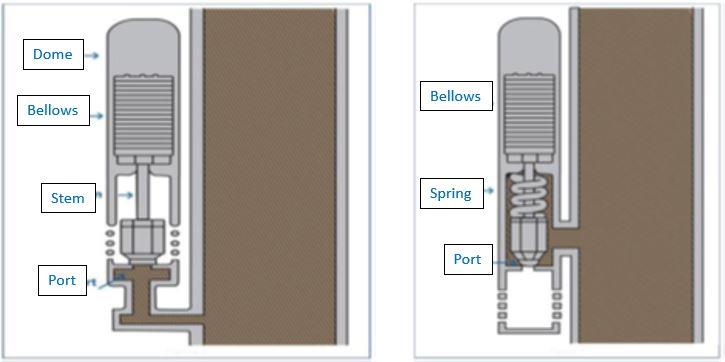
Figure 7: GLV (IPO and PPO respectively). There are two main forces that open a GLV: (1) injected gas pressure in the annulus and (2) produced fluid pressure in the tubing. As the gas being injected through tubing, the tubing pressure starts dropping. Therefore, the valve will close and stop gas flow from the annulus. In the case of a continuous flow system, only the operating valve remains open.
GLV Behavior Based on Flow Patterns
The behavior of each GLV under operating condition strongly depends on the injection gas pressure, the port size and the produced fluid pressure. The optimum performance of a GLV is when the valve operates under critical flow conditions in which the injection gas pressure is high enough to compensate the downstream fluid pressure and therefore maximum lifting production is achieved. Following are some flow behaviors through the GLV: Critical flow is defined as the state when the magnitude of the fluid stream velocity reaches sound velocity at the minimum flow area where, is supposedly the port area in a GLV. The pressure at the throat is the critical pressure (i.e. for air flowing under isentropic conditions this ideally 0.528 x injection pressure (𝑃𝑖)). Subcritical flow is when fluid stream velocity at the port is less than the sonic velocity or subsonic. Orifice flow is characterized by a region of increase in flow rate as the tubing pressure decreases until maximum flow rate is achieved. Once flow rate becomes maximum, any more pressure drop in the tubing pressure does not affect the fluid rate. In the orifice flow region, the injection pressure is high enough that the ball is lifted off the seat and minimum area open to flow is equal to the port area. Throttling flow region is characterized by a region of increasing flow rate as the tubing pressure is decreased until maximum flow rate is achieved. Then the flow rate through the valve decreases as the tubing pressure is decreased further. Transition flow region is characterized by a region of increasing flow as the production pressure is reduced. This region is followed by decreasing flow and then, constant flow as the production pressure is further reduced. The throttling and transition flow behaviors are caused by the nature of the compressible gas flow through the ball seat configuration. The flow of the gas in transition region determines the pressure profile on the ball, which is integrated over the ball area to determine the upward force acting on the ball. This force is divided by the area to determine the effective pressure. The change in area along the ball-seat configuration makes the ball-seat configuration analogous to a convergent-divergent nozzle Nieberding was the first to point out the gas passage through GLVs occurs mainly under two different flow patterns of throttling and orifice flow [11]. Throttling flow resembles flow through a variable area venturi; whereas orifice flow is very similar to gas flow through a fixed choke. Figure 9 depicts schematic performance curves in the gas rate against production pressure for these two flow patterns. The orifice flow model can be divided into two regions: subcritical and critical. At critical flow, flowing gas velocity across the valve port equals to the sound velocity, and injection rate remains at its maximum value regardless any further decrease in tubing pressure. This flow pattern occurs when the stem in the GLV at its maximum travel so the port area is the smallest passing flow area.
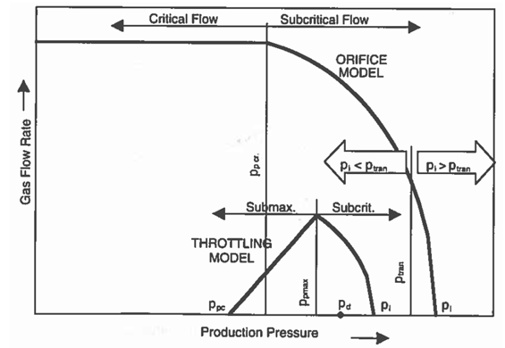
Figure 9: Schematic GLV performance for the orifice and throttling flow patterns. When the injection pressure (𝑃𝑖) is not enough to handle the closing pressure, the valve behaves in the throttling flow pattern. When the GLV behaves in the throttling flow pattern as the production pressure decreases, the gas flow rate increases due to an increase in the differential pressure across the valve seat. After reaching critical pressure point, flow rate decreases with further decreasing in production pressure until gas flow cease at the closing production pressure (𝑃𝑃𝐶).
GLVs Classifications
Depending on the gas lift applications, several types of GLVs can be deployed (Takacs, 2005). Some of the conditions upon selecting the right GLV for the application are listed as follows: 1. Mechanically controlled from the surface (by wireline, drop bar) 2. Other control methods include flow velocity, specific gravity, etc.
3. Pressure-operated valves get opened and closed by injection and /or production pressure. Mechanically controlled valves open and close from the surface by some mechanical means, most commonly by wire line. This type of the valves is used in intermitted lift wells; its biggest disadvantage is the unloading operation had to be accomplished manually. The specific gravity differential valve, on the other hand, was used for unloading continuous flow installations. Its main element is a flexible diaphragm that opens and closes the valve based on the pressures acting on its two sides. A control force is provided by a liquid charge of a set specific gravity, and the valve opens based on the actual fluid gradient at the valve depth. This valve proved to be an excellent option, however because of its bulkiness was later replaced by modern types.
Testing & Modeling
Different techniques are used to predict gas lift valve behavior. The Thornhill-Craver choke equation is the most used equation to predict gas lift valve performance. This equation was developed using the positive flow choke data. Many researchers used Thornhill-Craver equation to calculate the gas throughput and handled the gas lift valve as an orifice. Some other studies deliberated gas lift valve as a convergent-divergent nozzle and calculated the gas throughput accordingly. Neiberding and Acuna presented that the Thornhill-Craver’s equation often overestimate the performance of gas lift valves, specifically for the larger port sizes [11, 12]. Decker built analytical model to study the bellows operated gas lift valve behavior [13]. In his work, he investigated the effect of thermodynamic and mechanical factors in the pressure distribution and solved the force balance equation including these two factors. Thornhill-Craver equation did not consider the effect of gas compression in actual gas lift valve. The equation did not also treat the valve as a variable orifice. Winkler and Camp observed the effect of variable flow area [9]. They modified the Thornhill-Craver Equation 1 for variable area and gas compressibility.
155.5×Cd×Ae×P1√2g× K
K−1×{r2/K−r(K+1)/K}
√ZGT (1) Where: 𝑄𝑔𝑎𝑠= gas flow rate, Mscf/D 𝐶𝑑 = discharge coefficient 𝐴𝑒= Effectivearea of oriffice opening, sq inches 𝑃1 = upstream pressure, psi Qgas =
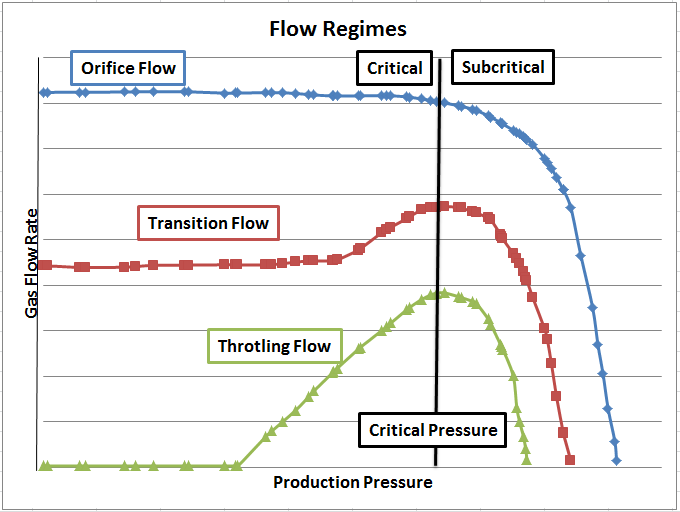
𝑃2 = down stream pressure, psi 𝑔 = acceleration of gravity, 32.2 ft/sq sec. 𝐾 = Cp/Cv spcific heat ratio 𝑟 = 𝑃2/𝑃1> ro ro = (2/K+1)^ k/(K-1) 𝑍 = comprisipility factor 𝐺 = specific gravity of gas ( air = 1) 𝑇 = inlet temperature of choke, R Winkler and Camp studied the valve performance considering the effect of the operating forces on bellows load rate and linear stem travel for many valves and they found that a simple mathematical model to predict gas lift valves is questionable due to the effect of these factors [9]. Also, they introduced the Benchmark valve to obtain the valve discharge coefficients (𝐶𝑑)which may be used to calculate the flow rate for actual gas lift valves. Decker pointed out that as the flow area changes, the 𝐶𝑑 also changes and cannot be used as a constant in Thornhill-Craver equation [14]. He also described the best technique to perform gas lift valve performance test. He discovered that the stem travel and opening and closing pressures cannot be calculated from static force balance. Based on control valve capacity test procedures he used flow coefficient (𝐶𝑣) concept instead of 𝐶𝑑 and presented flow coefficients as a function of stem travel. Tulsa University Artificial Lift Program (TUALP) started to study the gas lift system in 1983. An orifice and throttling flow models were built to define the gas passage through gas lift valve. The researchers created the flow performance family in orifice, transition and throttling flow as shown in Figure 10.
Bigilarbigi developed the facilities and procedures for valve testing [15]. He adjusted constant injection pressure test (CIPT). Based on the experimental result he built statistical model to simulate the flow performance of nitrogen and spring loaded valves and predict valve performance. An error in the static test facility made all his test data invalid. Nieberding corrected the static test facility error and developed statistic models for throttling and orifice flow based on test data [11]. He used the test rack opening pressure (𝑃𝑡𝑟𝑜) as a reference to distinguish between throttling and orifice flow. He pointed out that the valve behaves like an orifice if the injection pressure is above the test rack opening pressure. However, if the injection pressure becomes lower than the test rack opening pressure but greater than the valve closing pressure (𝑃𝑣𝑐), the valve will behave like a throttling valve. He also used methane as injected gas instead of air to examine his test procedure. In addition, he developed a correlation (2-2) to predict gas passage.
Pinj×(Pinj−Ppd)
(1−β4)×Tinj×Zinj×γg (2) Qgas = 1240.3 × Ap × Cd × Y√
Where,
Qgs = Gasthroughput, Mscf
d ;
Ap = Port area, in2; Cd = Discharge coefficient; Y = Gas expansion factor; Pinj = Upstream gas injection pressure, psig ; Ppd = Downstream gas injection pressure, psig ; β = Square root of ratio of port to inlet area ; Tinj = Temperature gas injection , R ; Zinj = Comprisibility factor at injection pressure ; γg = Gas specific gravity . Hepgülar established a mechanistic model to extensively decrease the number of tests that must be made to completely investigate the valve performance [16]. He modified Biglarbigi's test facility to measure the internal pressures and temperature during dynamic testing and stem movements and the load rate in static tests. He detected that when the gas flow rate exceeds 1.4 MMscf/d, the model was not as accurate as the empirical testing process. Acuña used Nieberding’s orifice flow model to normalize the valve data [12]. Rather than using a dynamic model he developed a statistical model. He also built another model for the throttling flow region. Sagar implemented both experimental and theoretical studies [17]. He tested pressure operated nitrogen gas lift valve (Merla make N-15R valve) and developed empirical equations quantifying bellows performance. He also developed a model using a Quasi-one dimensional flow theory for a convergent-divergent nozzle to explain the complex high velocity gas flow through the ball seat configuration. During his study he pointed out that pressure operated valve is sensitive to performance parameters. A small variation of 1% in injection pressure and temperature can change the maximum flow rate by as much as 30%. Rodriguez tested Nieberding and Acuña models at various pressures operated gas-lift valves to examine these models performance [18]. He developed empirical model and verified that constant production pressure test (CPPT) and the constant injection pressure test (CIPT) methods are equivalent for valve performance testing. Escalante developed a single equation model for orifice and throttling flow performance [19]. She described the ratio of the effective flow area (𝐴𝑒𝑓𝑓) to the port area (𝐴𝑃) as effective area factor ( 𝐴𝑓). She figured out that the relationship between 𝐶𝑑× 𝑌 × 𝐴𝑓and the valve’s throttling behavior is linear. For throttling flow, she introduced a new term, dimensionless stem position (𝑁𝑆) which is sensitive to changes in valves closing pressure. On the other hand, she used 𝐴𝑓 = one for orifice flow. The final form of gas passage equation was:
Piod×(Piod−Ppd)
Tv×Zv×Sg (3)
Qgs = 1240.3 × Ap × Cd × Y × Af√
Where,
Qgs = Gasthroughput, Mscf
d ;
Ap = Port area, in2;
Af = Aeff
;
Ap
Cd = Discharge coefficient; Y = Gas expansion factor; Piod = Upstream gas injection pressure, psig ; Ppd = Downstream gas injection pressure, psig ; Sg = Gas specific gravity . Bertovic accomplished comprehensive research [20]. He performed experimental and theoretical studies of the flow performance for one inch GLV. The model uses six coefficients to predict flow regimes, orifice, throttling and transition. To study GLV behavior, Faustinelli built a model for all three flow regimes [21]. To calculate volumetric flow rates through the valve, the model uses only four empirical parameters. Furthermore, Faustinelli developed a numerical model to study the effect of production and fluid temperature on bellows effectiveness. This model can be used to calculate the dome temperature by following equation, 𝑇𝑑= 0.3 × 𝑇𝑝𝑑+ 0.7 × 𝑇𝑖𝑛𝑗(4) Where, Td = Valve dome temperature, F; Tpd = Production fluid temperature, F; Tinj = Injection gas temperature, F; Both, Bertovic’s and Faustinelli’s models assumed one dimensional flow and the ball-seat area is only a function of the dimensionless stem position, which may not be accurate to use in transition flow. In their models, they used only three different valve closing pressures. So the calculated coefficient is not valid for other valve closing pressures. Shahri developed simple, rapid, and very inexpensive method to test the GLV in the critical flow region [4]. Also, he examined the effectiveness of Thornhill-Craver (TC) equation and corrected the equation for the discharge coefficient value. Another way to model the gas flow behavior is using numerical technique such as Computational Fluid Dynamics (CFD). CFD can be defined as the field that uses computer resources to simulate flow related problems. This field has been developing for the past 30 years. Due to the introduction of new computer specifications, the CFD has been used extensively. Before computational fluid dynamics was introduced, some scales were difficult to simulate. In 1930, two dimensional (2D) methods were established to solve the linearized potential equations using conformal transformations of the flow [22]. Richardson is the first one who introduced the earliest type of calculations for modern CFD [23]. Actually, his book "Weather prediction by numerical process," is the foundation for modern CFD and numerical meteorology. He used finite differences method and divided the physical space in cells. T3 group, a Consulting and Software Development Company developed three- dimensional method [24]. They used computers to model fluid flow using Navier-Stokes equations. In 1967 Hess published the first paper with three-dimensional model [25]. In their paper, they presented programs called Panel Methods which discretizes the surface of the geometry with panels. Turzoand Takacs developed a numerical solution for the GLV behavior that generated results in agreement with the API specifications [26, 27]. In their approach, they solved five sets of equations including Navier-Stokes equation, state of the fluid which in compressible, conservation of mass, energy, and the enthalpy changes due to change in internal energy at each position. The main caveat of this approach is associated with the correct assignment of pressure distribution pattern on the ball tip.
References
-
Brantly JE (1961) History of Petroleum Engineering. Boyed Printing Co, Dalals, Texas.
-
Cloud WF (1937) Petroleum Production. Norman: University of Oklahoma, pp: 613.
-
Brown KE (1984) The Technology of Artificial Lift Methods. Vol 2a, PennWell Publishing Company, Tulsa, Oklahoma.
-
Shahri MA (2011) Simplified and Rapid Method for Determining Flow Characteristics of Every Gas-Lift Valv. Texas Tech University, USA, pp: 1-128.
-
Pablano E, Camacho R, Fairuzo YV (2002) Stability Analysis of Continuous-Flow Gas-Lift Wells. Society of Petroleum Engineers, SPE Annual Technical Conference and Exhibition, San Antonio, Texas.
-
Bellarby J (2009) Well Completion Design. 1st (Edn.), 56: 726.
-
Fleshman R, Lekic HO (1999) Artificial Lift of High- Volume Production. Oilfield review, p: 48-63.
-
Osuji LC (1994) Review of Advances in Gas Lift Operations. Society of Petroleum Engineers.
-
Winkler HW, Camp GF (1987) Dynamic Performance Testing of a Single Element Unbalanced Gas-Lift Valves. Society of Petroleum Engineers, SPE Production Engineering, 2(3).
-
King W (1944) Time and Volume Control for Gas Intermitters. US Patent No. 2,339,487.
-
Nieberding M (1988) Normalization of Nitrogen Loaded Gas-Lift Performance Data. The University of Tulsa, Tulsa, pp: 267.
-
Acuna HG (1989) Normalization of One Inch Nitrogen Charged Pressure Analysis Gas-Lift Valves. Chapter VI, pp: 251.
-
Decker AL (1976) Analytical Methods for Determining Pressure Response of Bellows Operated Valves. Society of Petroleum Engineers.
-
Decker KL (1986) Computer Modeling of Gas-Lift Valve Performance. Offshore Technology Conference, Houston, Texas.
-
Biglarbigi K (1985) Gas Passage Performance of Gas- Lift Valves. Tulsa, pp: 206.
-
Hepguler G (1988) Dynamic Model of Gas-Lift Performance. The University of Tulsa, Tulsa, pp: 179.
-
Sagar R (1991) An Improved Dynamic Model of Gas- Lift Valve Performance. The University of Tulsa, Tulsa, pp: 217.
-
Rodriguez M (1992) Normalization of Nitrogen- Charged Gas-Lift Valve Performance. The University of Tulsa, Tulsa, pp: 151.
-
Escalante S (1994) Flow Performance Modeling of Pressure Operated Gas-Lift Valves. The University of Tulsa, Tulsa, pp: 104.
-
Betrovic D, Doty D, Blais R, Schmidt Z (1997) Calculating Acurate Gas-Lift Flow Rate Incorporating Temperature Effects. Society of Petroleum Engineers, SPE Production Operations Symposium, Oklahoma.
-
Faustinelli JG, Doty DR (2001) Dynamic Flow Performance Modeling of a Gas-Lift Valve. Society of Petroleum Engineers, SPE Latin American and Caribbean Petroleum Engineering Conference, Buenos Aires, Argentina.
-
Thomson LM (1973) Theoretical Aerodynamics. 4th (Edn.), Dover Publications, New York.
-
Richardson LF (1965) Weather Prediction by Numerical Process. Dover Publications, pp: 1-27.
-
Harlow FH (2004) Fluid Dynamics in Group T-3 Los Alamos National Laboratory. Journal of Computational Physics 195(2): 414-433.
-
Hess JL, Smith AMO (1967) Calculation of Potential Flow about Arbitrary Bodies. Progress in Aerospace Sciences 8: 1-138.
-
Turzo Z, Takacs G (2009) Special Report: CFD techniques determine Gas-Lift Valve Performance. Oil & Gas Journal.
-
API (2001) Recommendation Practice Gas-lift Valve Performance Testing. 2nd (Edn.), API RP 11V2.
-
API (1994) Gas Lift Manual book 6. 3rd (Edn.), Exploration and Production Department, API, USA.
-
Brown KE (1967) Gas Lift Theory and Practice. Englewood Cliffs NJ, Prentice-Hall, pp: 924.
-
Economides MJ, Hill AD, Ehlig-Economides C, Zhu D (2012) Petroleum Production Systems. 2nd (Edn.), Prentice Hall, pp: 1-730.
-
Encycloedia CE (2013) Coanda Effect. 6th (Edn.).
-
Kulkarni M (2005) Gas Lift Valve Modeling with Orifice Effects. Texas Tech University, Lubbock, Texas.
-
Takacs G (2005) Gas Lift Manual. Pennwell Corporation.
- Nigeria’s Vulnerability in the Face of Global Energy Policy
- A Simulation Study of Investigation of Optimum Oil Production Performance by Applying Various Gas Injection Methods in Oil Reservoir
- Characterization of Permo-Triassic Reservoirs through Thermal Maturity Assessment of Westphalian Source Rocks in the Cheshire Basin
- Influence of Microwax on the Rheological and Thermal Behaviour of a Wax Crude Oil
- Real-Time Monitoring and Performance Optimization of Steam Injection in Heavy Oil Reservoirs Using Fiber Optic Sensing and Integrated Predictive Simulation Models
- Rapid On-Site Determination of the Total Petroleum Hydrocarbon Content of Soils by Handheld Fourier Transform Near-Infrared Spectroscopy: Development of a Global, Site- and Scanner- Independent Calibration Model