Real-Time Monitoring and Performance Optimization of Steam Injection in Heavy Oil Reservoirs Using Fiber Optic Sensing and Integrated Predictive Simulation Models
Real-time surveillance that identifies departures from safe operating limits and permits timely remedial action is essential to effective reservoir management. This study uses distributed fiber-optic sensing (FOS) to assess the effectiveness of steamassisted gravity drainage (SAGD) in Suplac Field, a heavy-oil reservoir (8–13 °API, 500–1000 cP). Wells #1 and #2, two horizontal injectors, are observed for two full steam-injection cycles that lasted 130 and 150 days, respectively. Together with downhole pressure and steam-quality measurements, high-resolution FOS data yielded 3D temperature profiles down the wellbore, which were then analyzed to determine out-of-range operating situations and quantify reservoir reaction. Comparisons across cycles showed how temperature fronts changed, how steam quality deteriorated, and how output indicators like water cut and oil rate drop changed. In order to estimate temperature, pressure, and steam quality under the same injection settings, a linked wellbore/reservoir model was constructed in Prosper to simulate fluid characteristics in the tubing and annulus. The methodology was validated and areas where real-time FOS data might improve simulation assumptions were highlighted by the model outputs' reasonable agreement with FOS observations. An effective method for optimizing heavy-oil steam injection that improves recovery efficiency and operating safety is the combined FOS–simulation approach.
Introduction
After primary and secondary recovery, enhanced oil recovery (EOR) is usually the last stage of oil production. While secondary recovery uses water injection to sustain pressure when natural energy diminishes, primary recovery depends on the reservoir’s natural pressure or artificial lift to extract oil. Tertiary recovery, or EOR, is used when these techniques become economically inefficient, frequently as a result of increased water output. EOR increases oil output by extracting more oil using thermal, chemical, or other means. EOR can be utilized at any point when conventional techniques are inadequate, even though it is often utilized near the end of a field’s life [1]. The two main procedures in thermal EOR are steam stimulation (cyclic steam injection) and steam-flooding. Steam and hot-water flooding are the predominant approaches. These techniques improve flow to producing wells by decreasing the viscosity of heavy oils. The most efficient EOR technology is steam-flooding, which recovers around 410 million barrels of oil per day worldwide. In-situ combustion and steam stimulation recover 57 million barrels per day, while all other EOR techniques recover 220 million barrels per day [2]. Heavy oil production frequently uses thermal EOR, which includes steam injection methods including In-Situ Combustion (ISC), Cyclic Steam Stimulation (CSS), and Steam Assisted Gravity Drainage (SAGD). The geographic resolution of traditional monitoring systems is frequently restricted. Distributed, real-time temperature and acoustic data collecting along the whole wellbore has been made possible by the advent of Fiber Optic Sensing (FOS), namely Distributed Temperature Sensing (DTS) and Distributed Acoustic Sensing (DAS) [3, 4].
The fundamental idea of a FO system is based on a transmitted light signal in which the FO cable (measured light) acts as a carrier for light, sending out a light signal from the transmitter on the surface. Reflected light is produced by light pulses and has an extremely low attenuation index. In order to reach the receiver at the surface, the backscattered light waves must return via the optic medium. The data is decoded, or converted to temperature, pressure, acoustic, or strain data, and then recorded in a database based on the technology used. This process compares the backscattered light signal with the light pulse that was first fired from the transmitter (reference beam). FOS Techniques are widely applicable in thermal EOR. There are two technologies for FOS operations. DTS Technique is the initial technique. Raman scattering in optical fibers is used by the DTS technology to monitor temperature profiles [3]. In SAGD operations, DTS has been very helpful in tracking the growth of the steam chamber and optimizing the SOR [5]. Field research conducted in Alberta showed how DTS was able to record the steam chamber’s temporal development, allowing for modifications in steam injection to increase the effectiveness of oil recovery [5]. The second is DAS, which uses Rayleigh backscattering to create continuous acoustic sensors out of optical fibers [6]. By offering dynamic flow monitoring, DAS enhances DTS. DAS applications for detecting steam flow patterns during injection in thermal EOR processes were demonstrated by Mateeva, et al. [6]. A multi-physics sensing platform is provided by hybrid DTS/ DAS systems, which combine DTS and DAS [7]. According to recent advancements, integrated fiber systems can increase reservoir interpretation and control by providing temperature, acoustic, and strain data [7, 8].
FOS Applications in Thermal EOR Methods are several. DTS makes it possible to track the compliance of the steam chamber in SAGD wells in real time, which helps to prevent steam channeling and optimize production techniques [9].
Operators may dynamically modify steam injection profiles thanks to continuous feedback from DTS, which lowers heat losses and enhances SOR [9]. DTS has also been used in CSS projects to track the steam soak phase and evaluate production-related thermal behavior [10]. This type of monitoring optimizes following cycles and enables the identification of thermal inefficiencies [10]. Nonetheless, DTS detects sharp temperature gradients that correlate to combustion zones in ISC operations in order to follow thermal fronts [11]. According to field findings, DTS assists operators in tracking the combustion process and modifying injection plans as necessary [11].
Challenges in FOS Deployment for Thermal EOR represent a key-element during applications. Despite its benefits, FOS has certain drawbacks, most notably fiber deterioration at temperatures above 300°C [12]. Furthermore, logistical and financial challenges arise due to the intricacy of installation in horizontal or deviated wells [13]. Moreover, sophisticated machine learning algorithms are needed to analyze the enormous volumes of data produced by DTS/DAS [14]. Using digital twins and machine learning in conjunction with FOS data to automate decision-making is one of the emerging trends [15]. In order to improve sensor survival for prolonged thermal EOR operations, research on high-temperature fiber coatings is also ongoing [16]. Furthermore, the development of 4D monitoring systems for subsurface operations appears to be promising when DTS, DAS, and DSS are applied together [17].
For better understanding the field monitoring and evaluation philosophy, it is advisable to know the best way to measure the changed parameters, how to measure them, and their effect on all field studies including wells and reservoir. By comprehending the observed variables and suggesting remedial action in real time, reservoir management seeks to maximize process efficiency in the reservoir. One crucial component of production facilities that might endanger the safe growth of a project is the detection of out-of-range operating situations. During injection and production cycles, continuous real-time temperature and pressure monitoring for heavy and viscous oil well production optimization aids in the optimization and improvement of CSS scenarios, provides information about heat transfer by convection and conduction into the reservoir, records any breakthroughs in steam or water, records any evidence of combustion gas breakthroughs, enhances comprehension of the processes occurring inside the borehole (downhole), and provide information for reservoir modeling and other optimization strategies.
Therefore, the main objective of this paper is to investigate temperature-pressure distribution using FOS in Suplac field wells during injecting a steam into a heavy crude oil reservoir. Two horizontal drilled wells are used in injecting steam into the reservoir. Two complete injection steam cycles are done for each, 130 and 150 days for well # 1 and 2 respectively. A comparison study between the two cycles is done for both well including pressure, temperature, steam quality, production parameters over the specified period. In addition, a model is developed using Prosper software to predict the fluid well, tubing and annuli temperature and pressure, and steam quality for steam injections with certain parameters. Thus, it is important to review the FOS applications, and EOR improvements. The Suplac field data are also described. Wells # 1 &2 data are described as well. Results and discussions are made.
A Chronological Review of Fiber Optic Sensing in Oil and Gas Fields
Thermal EOR monitoring capabilities have been significantly enhanced by FOS, especially DTS and DAS [3, 4]. FOS technologies are essential to creating intelligent, effective, and sustainable thermal EOR systems because of developments in fiber durability and AI-driven analytics [18]. In order to continue researching and apply FOS methods efficiently, a sequential review is made to study the historical studies, approaches, applications techniques of FOS especially in oil and gas field as shown in Table 1.
| Author | Published Year | Study/Approach/Technique/ Methodology/Application/Field Study |
|---|---|---|
| Early Developments and Establishments | ||
| Culshaw [19] | 2005 | Presenting the study that demonstrated the early idea of using FOS with health systems for critical infrastructure Distributed sensing was highlighted in Culshaw’s discussion of the growing potential of FOS in structural health monitoring |
| Measures [20] | 2006 | Investigating phase sensitivity in interferometric FOS. A fundamental grasp of several interferometric methods that are essential for precision sensing was given. |
| Kersey [21] | 2007 | Reviewing FBG sensors for structural applications in a groundbreaking manner. The scalability of FBGs for multiplexed sensing in huge structures was highlighted in his work. |
| Rao, et al. [22] | 2008 | Emphasizing strain monitoring while concentrating on FOS for aeronautical constructions. In challenging aeronautical settings, they illustrated the benefits of FO over conventional electrical sensors. |
| Bao & Chen [23] | 2010 | Introducing DTS applications in oil and gas in which the groundwork for using DTS in well integrity and production optimization was presented. |
| Growth into Distributed Sensing and Oil & Gas | ||
| Hartog [24] | 2011 | Examining downhole DAS applications. For DAS technology used in underground energy businesses, this work was a foundational resource. |
| Soto, et al. [25] | 2012 | Developing a real-time DTS for monitoring geothermal reservoirs. Their invention gave operators the ability to dynamically map temperature changes in geothermal areas. |
| Masoudi & Newson [26] | 2013 | Presenting recent developments in vibration sensors for distributed optical fibers. They showed how structural vibrations might be detected across long distances using FOs. |
| Liehr, et al. [27] | 2014 | Presenting a new optical frequency domain reflectometry (OFD) technique for dispersed sensing with greater resolution. By enabling sub-centimeter resolution measurements, OFD advanced the accuracy of distributed sensing. |
| Froggatt & Moore [28] | 2015 | Investigating DS using Rayleigh with enhanced spatial resolution. Using common telecom fibers, their technique enabled extremely precise distributed strain and temperature measurements. |
| Methods of High Resolution and Diversity of Sensing | ||
| Zhan, et al. [29] | 2016 | Creating strain sensors using FOs that have better multiplexing capabilities. By enhancing sensor multiplexing, the study made it possible to install dense sensors for structural health monitoring. |
| Parker, et al. [30] | 2017 | Transforming geophysical surveys by demonstrating DAS for seismic applications. Their innovation demonstrated that dense seismic arrays might be created from already-existing FO networks. |
| Selker, et al. [31] | 2018 | Expanding DTS uses in agriculture and hydrology. This study demonstrated DTS’s adaptability by demonstrating its use in irrigation management and soil moisture monitoring. |
| Zhang, et al. [32] | 2019 | Presenting the combined FOSs for temperature and pressure monitoring at the same time. They demonstrated how to integrate sensors for intricate settings like deep-water wells. |
| Fidanboylu & Efendioglu [33] | 2020 | Outlining novel construction techniques and materials for FSs. Advances in sensor design, such as new polymer coatings for enhanced sensitivity, were covered in detail in this study. |
| New Developments and Future Prospects | ||
| Farhadiroushan, et al. [34] | 2021 | Addressing the DAS in distributed strain imaging for CO2 sequestration monitoring. The potential of DAS in identifying tiny strain signals linked to carbon storage integrity was demonstrated by their work. |
| Smith & Farahi [35] | 2022 | Developing FOS devices that combine Raman scattering with FBG. The goal of this hybridisation was to solve the trade-off that FO devices face between sensing range and spatial resolution. |
| Wang, et al. [36] | 2023 | Presenting an improved understanding of FOS data using machine learning. The interpretation of massive datasets produced by dispersed sensors was greatly enhanced by machine learning techniques. |
| Xu, et al. [37] | 2024 | Building ultrafast FOS for high-speed rail structural integrity monitoring. Predictive maintenance was made possible by their system, which gave vital infrastructure real-time notifications. |
| Huang, et al. [38] | 2025 | Revealing advances in the use of innovative photonic crystal fibers for distributed sensing spatial resolution. This development opened up new possibilities for precise monitoring by pushing spatial resolutions to previously unheard-of limits. |
Table 1: A review of FOS techniques and application.
Study Methodology and Research Procedures
The goal of the project is to combine coupled wellbore– reservoir simulation with real-time distributed FOS in order to measure and optimize SAGD performance in the Suplacu heavy oil field. Early detection of out-of-range operating situations, optimization of the steam injection method, and enhancement of recovery efficiency while maintaining well integrity are the objectives.
Experimental Design
Two horizontal injector wells, Well #1 and Well #2, each outfitted with DTS and DAS systems to track SAGD performance, will be used in a field project in the Suplacu heavy-oil field as part of the experimental design. Near- continuous thermal and acoustic profiling of the wellbores is made possible by Well #1’s 24 DTS sensors and one pressure gauge and Well #2’s 14 DTS sensors and one pressure gauge. With baseline injection rates of 90 t/d for Well #1 and 55 t/d for Well #2, both wells go through two full SAGD cycles (130 and 150 days) under controlled steam injection programs, with wellhead conditions of 12–13 bar and 220°C. Throughout the project lifespan, the setup supports integrated monitoring and model calibration by simulating real-time field operations and enabling real-time data gathering on temperature, acoustic signatures, pressure, flow rate, water cut, and steam quality.
DataAcquisition Protocol
- Installation & Calibration • Install armored optical cables beneath the casing; during cold shut-in, conduct a baseline DTS/DAS assessment. • Adjust the FO temperature at three depths in relation to the reference platinum RTDs.
- Live Injection/Production Logging • Stream data to office servers via RMDA (resolve previous 1 s overlap issue by aligning acquisition to 10 min cadence); record DTS every 10 minutes and DAS every 1 minute.
Modelling & Analysis Workflow
- Record synchronous P-T-Q data from the wellhead. 3. Quality Control
- Perform automated detection of sensor drift and dropouts > 0.2 bar or > 3 °C; initiates field check within 24 hours.
- Prevent the previously mentioned data gaps by maintaining a backup power source.
| Step | Action |
|---|---|
| Coupled Simulation | Build Prosperlinked wellbore/reservoir model; input measured rock/fluid properties (sandstone 2.65 g cm⁻³, k = 1.06 BTU hr⁻¹ ft⁻¹ °F⁻¹; heavy oil μ = 500–1 000 cP, 8–13 °API). |
| History Matching | Iteratively tune thermal conductivity, nearwellbore permeability and steamquality curve until simulated P–T envelopes converge to FO data within ±5 °C and ±0.5 bar. Address prior mismatch by adjusting gascap heat capacity and gauge bias. |
| RealTime Diagnostics | Apply machinelearning anomaly detector on DTS to flag steam breakthroughs, channelling or aquifer coning (e.g., persistent > 20 °C gradient over 10 m). |
| Optimization Loop | Every 30 d, recompute steamoil ratio (SOR), predict nextcycle steam allocation, and update Prosper boundary conditions. |
Table 2: Steps of model and study analysis.
Validation & Performance Metrics
- Thermal Front Tracking: Crossplot measured vs. simulated 3D temperature isotherms; target R² > 0.9.
- Production Response: Compare predicted and actual oil rate, water cut, and cumulative liquids; accept error ≤ 10 %.
- Steam Quality: Validate downhole quality (goal 70– 80 %) against Prosper outputs; reconcile if FO indicates subcooled water injection.
Work Procedures (Stepwise)
- Project Kickoff & HSE review (Week 0–1)
- Fiberoptic installation & baseline survey (Week 2–4)
- Cycle 1 steam injection & live monitoring (Day 0–130/150)
- Cycle 1 data cleanup, QC and preliminary model match (parallel, monthly)
- Intercycle analysis & parameter update (2 weeks downtime)
- Cycle 2 steam injection with optimized schedule
- Comprehensive history match and sensitivity study (postCycle 2, 4 weeks)
- Decision workshop—steam strategy and sensor expansion
- Final report submission This concise methodology leverages continuous FOS data to close the loop between field observations and predictive simulation, providing a robust framework for optimizing heavyoil steam injection in Suplacu and analogous reservoirs.
Field Data Description: Suplacu Heavy Oil Field
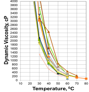
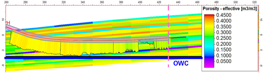
Suplacu field is an onshore oil reservoir produced heavy oil. In addition, it one of Romania’s oldest and most significant crude oil reservoirs and it is situated in Bihor County, close to the Hungarian border. Due to the production of heavy and viscous oil, which is a feature of mature deposits, exploitation started in the 1960s. The data is divided into many sections to depict the technical aspects of this field. First of all, it is situated in Bihor County, in the northwest of Romania. The field is situated at an average elevation of 180–220 meters across a mountainous terrain. Second, this mature field was identified in the 1960s, according to geological data. Neogene (Pliocene) formations are the source of the productive strata. Low permeability and high hydrocarbon saturation are characteristics of porous sandstone formations that contain crude oil. The productive layer ranges in depth from around 600 to 1000 meters. Third, the type of produced fluid is heavy crude oil. It is characterized by low API grade (8–13° API), high viscosity (at reservoir temperature, more than 500–1000 cp), and it includes significant levels of paraffin, sulfur, and asphalt[39]. Figure 1 shows the variation of oil viscosity with temperature from different wells. Fourth, Recovering and Exploiting Among the techniques are traditional primary exploitation through rod pumps and progressive cavity pumps (PCPs). The reservoir yields Low production because to the crude oil’s high viscosity.
Tertiary and Secondary Recovery (EOR): In vertical wells, CSS, was used. An industrial project using SAGD on two horizontal wells was also implemented and the hot water and/or superheated steam injection were used. Figure 2 demonstrates the history of recovery mechanisms until reaching to EOR.
Infrastructures include plants that produce steam, separators for oil and water and fluid heating systems, and pipes for injection and extraction that are thermally insulated. The historical production data shows that the average daily production rate (per active well) is 3–10 m³. Despite its advanced decline, the field had previously produced approximately 10 million tonnes of crude oil. The first PCP metal pumps, which can tolerate temperatures beyond 150°C, were used in Romania. Fiber optic sensors were also used for measuring SAGD well pressure and temperature in order to monitor the injection and reservoir temperatures in real time. Maximum bottom hole temperature (BHT), in steam injection phase is 230oC (446 oF), and the maximum Wellhead Temperature (WHT) is 250°C.
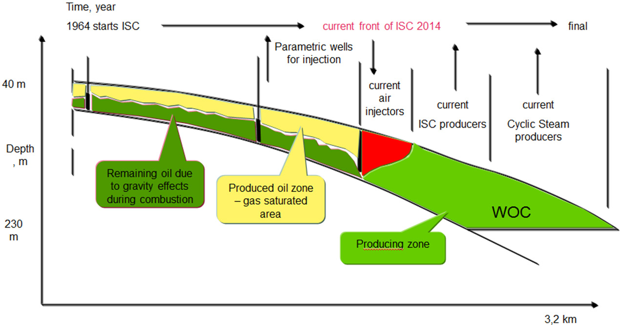
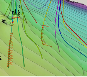
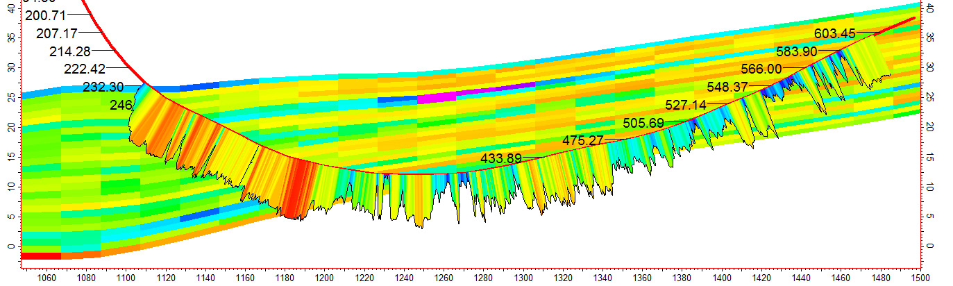
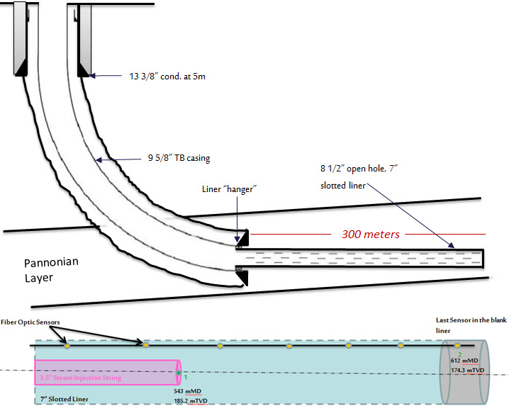
Figure 3: Structural map with drilled wells and FOS wells 1 and 2 used in steam injection. Data gathering & Data analysis of FOS Application Two wells, well #1 (24+1 sensors) and well #2 (14+1 sensors), each on a separate cluster (PAD), have fiber optics installed. Flexible interfaces are readily set up to deliver downhole data to the office system and facilitate communication between the site and the surface data gathering system. A field developed model update resolved the problem with the remote monitoring data acquisition (RMDA) system, where the data acquisition frequency was set at one second and some data was not recorded because of wavelength overlap. The RMDA system is set up at the same frequency as the system office, which has a 10-minute data acquisition frequency. Data analysis includes examination of CSS design and other downhole steam injection circumstances. The amount of steam and the duration of steaming are determined by field experience; When to shut down the well for a fresh CSS, minimum wellhead temperature for a new steam cycle or minimum oil output; There is no link between the steam table and the wellhead characteristics. Next, Questions to pose: Where does water production The following pictures, which come from a thermal simulation or monitoring system during steam injection, display the temperature distribution along a wellbore profile for well # 1 and 2. The well trajectory covered in grey is a horizontal profile on the color map, which shows temperature intensity with cooler areas in blue/green and hotter areas in red/orange. The well path’s labeled values emphasize heat dispersion and possible steam breakthrough or channeling by displaying temperature readings at different recorded depths (Figures 4 & 5). In the horizontal wellbore profile, the 9 5/8” casing is close to base reservoir until an inclination of 93+˚ (parallel to reservoir). Horizontal slotted liner is placed in open hole through the oil sands zone (Figure 6). Steam injection is done through a 3 1/2” tubing, thermal expansion joint and thermal packer. The oil production is performed through conventional rod pump.
| Type of fluid | Fluid Specific Gravity (SP. Gr) | Fluid Conductivity (BTU/hr/ ft/F) | Fluid Specific Heat Capacity (BTU/lb/F) |
|---|---|---|---|
| Water (Salinity<10000) | 1.00 | 0.35 | 1.00 |
| Water (Salinity<200000) | 1.08 | 0.345 | 1.02 |
| Water (Salinity>200000) | 1.15 | 0.34 | 1.04 |
| Heavy Oil | 0.96 | 0.083 | 0.49 |
| Medium Oil | 0.90 | 0.0825 | 0.50 |
| Light Oil | 0.84 | 0.0815 | 0.50 |
| Gas | 0.01 | 0.0215 | 0.26 |
| Type of Rock | Rock Density (g/cc) | Fluid Conductivity (BTU/hr/ ft/F) | Fluid Specific Heat Capacity (BTU/lb/F) |
| Sandstone (S.S) | 2.65 | 1.06 | 0.183 |
| Shale | 2.40 | 0.70 | 0.224 |
| Limestone (L.S) | 2.71 | 0.54 | 0.202 |
| Dolomite | 2.87 | 1.00 | 0.219 |
| Halite | 2.17 | 2.80 | 0.219 |
| Anhydrite | 2.96 | 0.75 | 0.265 |
| Gypsum | 2.32 | 0.75 | 0.259 |
| Lignite | 1.50 | 2.00 | 0.30 |
| Volcanic | 2.65 | 1.60 | 0.20 |
| Fixed Value | 2.61 | 1.10 | 0.20 |
Table 3: Fluid and rock properties used in modelling.
Field Results and Discussions: Real Time Measurements, Simulations and Comparisons
Real-time surveillance that identifies departures from safe operating limits and permits timely remedial action is essential to effective reservoir management. This study uses distributed fiber-optic sensing (FOS) to evaluate the effectiveness of SAGD in Suplacu Field with a heavy oil reservoir of 8–13 °API, and 500–1000 cp viscosity. Wells #1 and #2, two horizontal injectors, were observed for two full steam-injection cycles. Table 3 shows the rock and fluid properties of Suplacu reservoir that were used during modeling with prosper. Figures 1 through 6 show the field map, well profile and data used in this study.
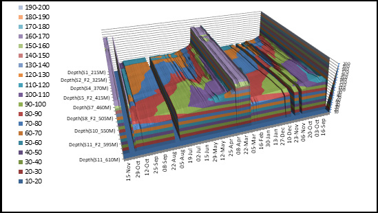
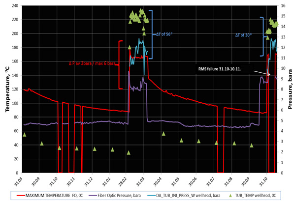
The temperature distribution in a well over time – almost one year– and depth is depicted in the 3D graph shown in Figure 7, most likely during a steam injection or other thermal recovery procedure. The z-axis displays temperature oC, colour-coded in bands (from 90–100°C up to 190–200°C), the y-axis displays depth at different sensor sites (varying from ~215 m to ~610 m), and the x-axis depicts time (from mid-November to mid-September). The temperature zones’ contours and layers indicate changes in heat penetration at various depths and periods as well as the movement of the thermal front. Temperature profile spikes and plateaus signify active steam injection times, well shut-in times, or injection technique adjustments. For tracking thermal efficiency and seeing heat breakout zones or steam channeling over time, this visualization is helpful. FO-based temperature and pressure monitoring in well #1 throughout a year of steam-assisted gravity drainage (SAGD) operations is shown in Figure 8. Sharp rises in wellhead injection pressure (up to about 13.5 bar) and accompanying temperature spikes reaching 220°C, with ΔT values of 56°C and 30°C, emphasize two main steam injection cycles. Effective steam propagation is shown by steady baseline conditions and distinct heat and pressure responses during injection, as shown by FO data. Additionally, the graphic shows a short loss of data due to an RMS (Remote Monitoring System) breakdown that occurred over a period of 1.5 years. All things considered, the figure illustrates how FOS makes it possible for ongoing downhole monitoring for real-time diagnostics, well integrity evaluation, and thermal EOR optimization.
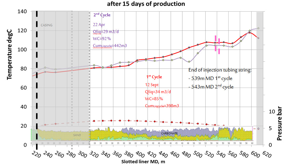
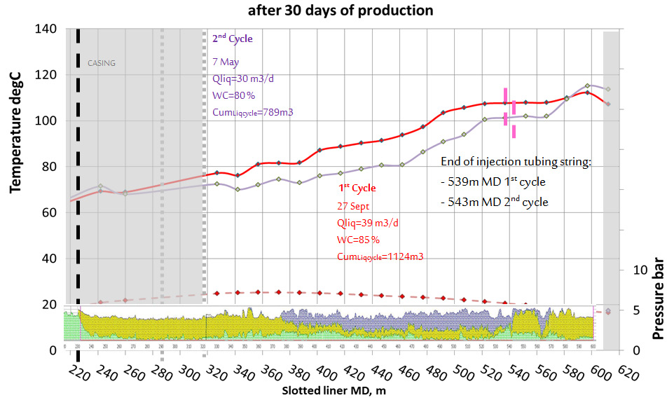
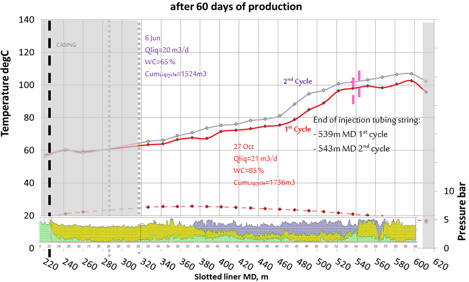
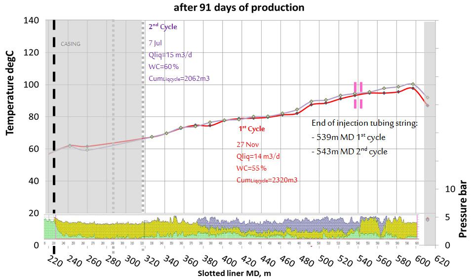
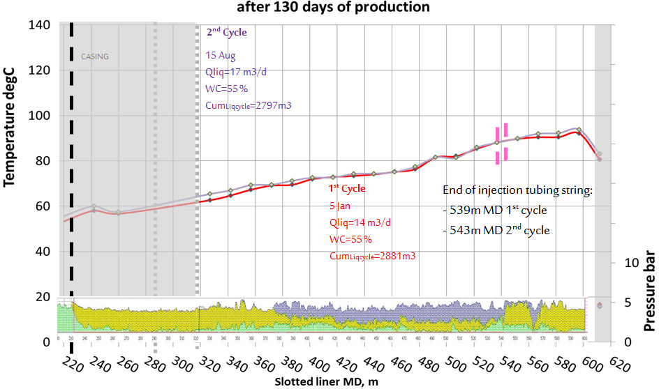
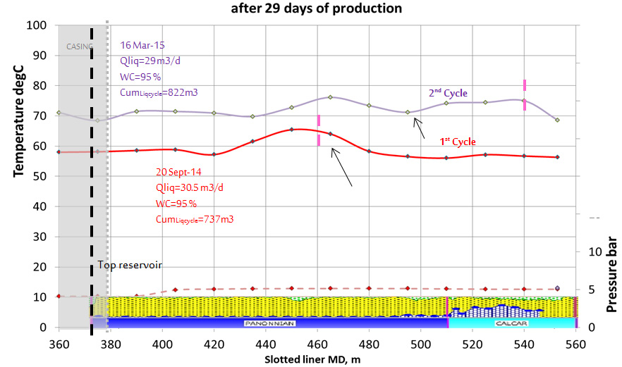
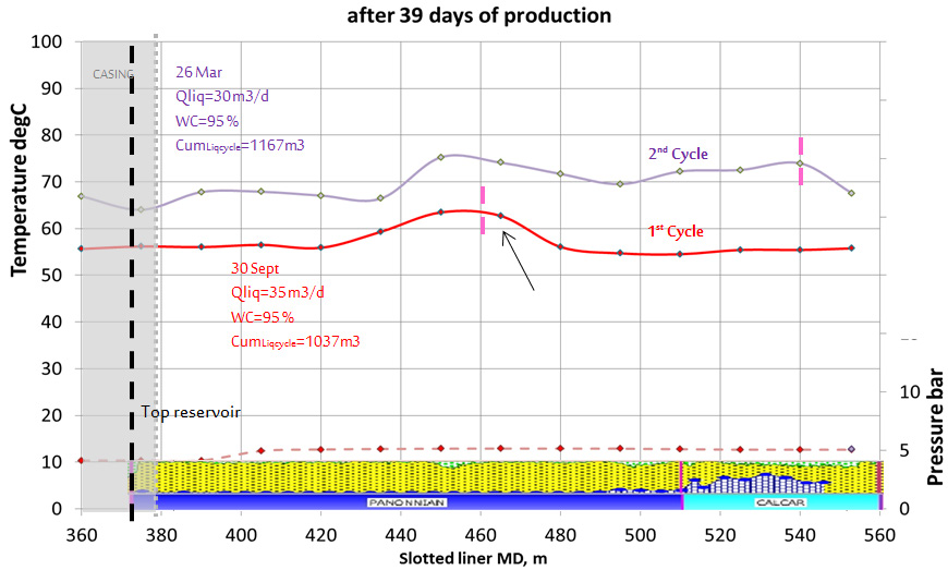
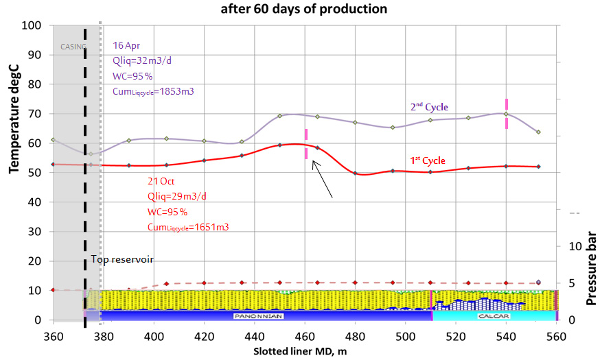
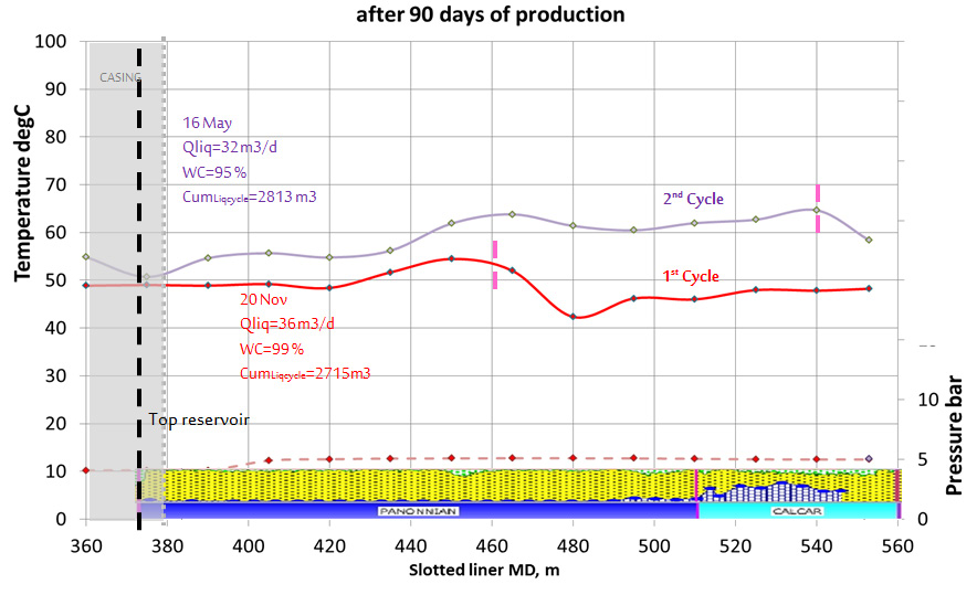
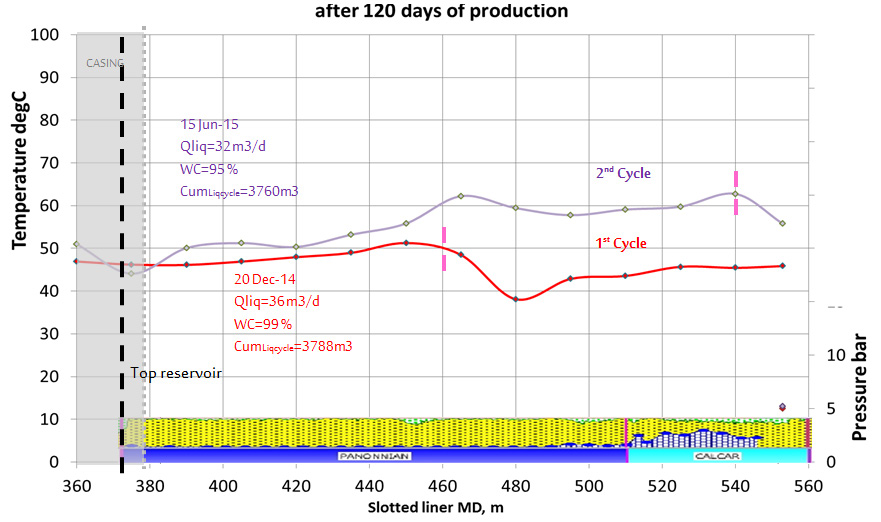
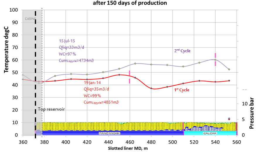
Figures 9 through 13 show how temperature and pressure changed throughout the course of 130 operating days along a slotted liner, signifying two production cycles. The five graphs, which are divided into different stages— after 15, 30, 60, 91, and 130 days—show the temperature and pressure behavior along a slotted liner in a wellbore during the period of 130 days of production. Temperature (°C) and pressure (bar) are shown against the slotted liner’s measured depth (MD) in each graph. Interestingly, two manufacturing cycles are recorded; the first is often indicated by red text, while the second is shown by purple. Water cut (WC) and liquid production rate (Qliq) are monitored for each cycle as production time goes on, and cumulative liquid production is shown to measure reservoir performance. Along with the injection tubing termination sites for each cycle, the graphs also indicate important completions and formations like “SAND” and “CARBONATE”. The temperature profile gradually decreases over the course of the five time periods, particularly in the vicinity of the well’s toe (in the direction of greater MD), suggesting thermal front movement brought on by production drawdown and cooling by produced fluids. Higher Qliq and WC values are first seen, particularly in the second cycle. But with time, WC improves as Qliq declines, indicating better oil cut as water output declines. By day 130, WC is at 55% and Qliq for both cycles is between 14 and 17 m³/d. The pressure seems to stabilize at 5 bar or less, and the temperature becomes more consistent. As is common in thermal recovery operations, the data show front stabilization, production drop, and reservoir cooling. A mature thermal sweep and decreased thermal losses are implied by the improvement in WC and comparatively stable temperatures at later stages, which suggest a manufacturing regime that is steadily stabilizing.
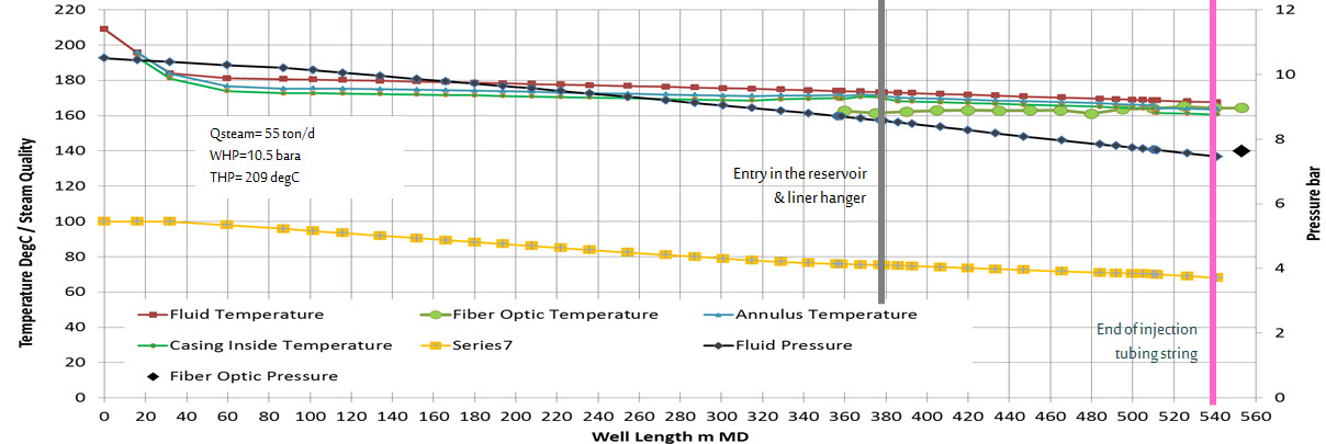
The next graphs (Figures 14&15) show the temperature and pressure profiles along a wellbore during steam injection as observed by FO and modeled (Prosper). The y-axes display pressure (right) and temperature/steam quality (left), while the x-axis shows the well length (in measured depth). In both pictures, temperature, steam quality, and pressure are shown versus measured depth, comparing calculated Prosper outputs with measured FO data for Well #1 during steam injection. The graphs provide a number of temperature profiles, such as FO, Prosper fluid, annulus, and casing temperatures, in addition to Prosper-calculated fluid pressure and steam quality. Important well components, such as the liner hanger, casing shoe, and injection tubing string end, are indicated by comments. One noteworthy finding in both figures is that, as the FO data suggests, Prosper model overestimates temperatures above the reservoir. The results also demonstrate the steam entering the reservoir at about 220 m MD and indicate constant injection circumstances (90 tons of steam per day, WHP = 12.84 pressure, THP = 220°C). In model 1, it is possible that the reservoir temperature is warmer than initially because of gases from combustion + previous steam cycles. In this model, the pressure is reasonably matched, but the temperature is off. Also, it was not possible to derive a model with both matched (Figure 14). In the second model (Figure 15), the temperature is matched, but the pressure is not matched. Also, Prosper will predict saturation conditions, which was not what was recorded. In both unmatched models, the calculated steam quality is ~80%.
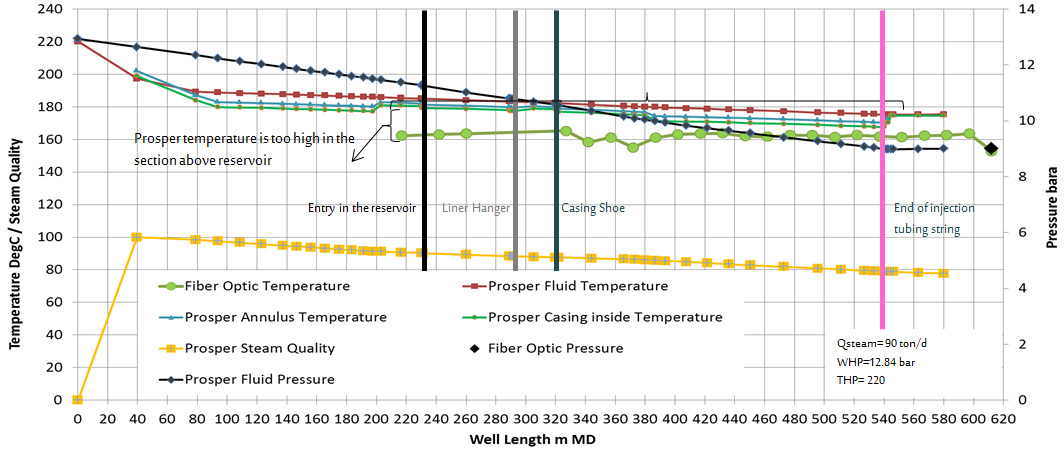
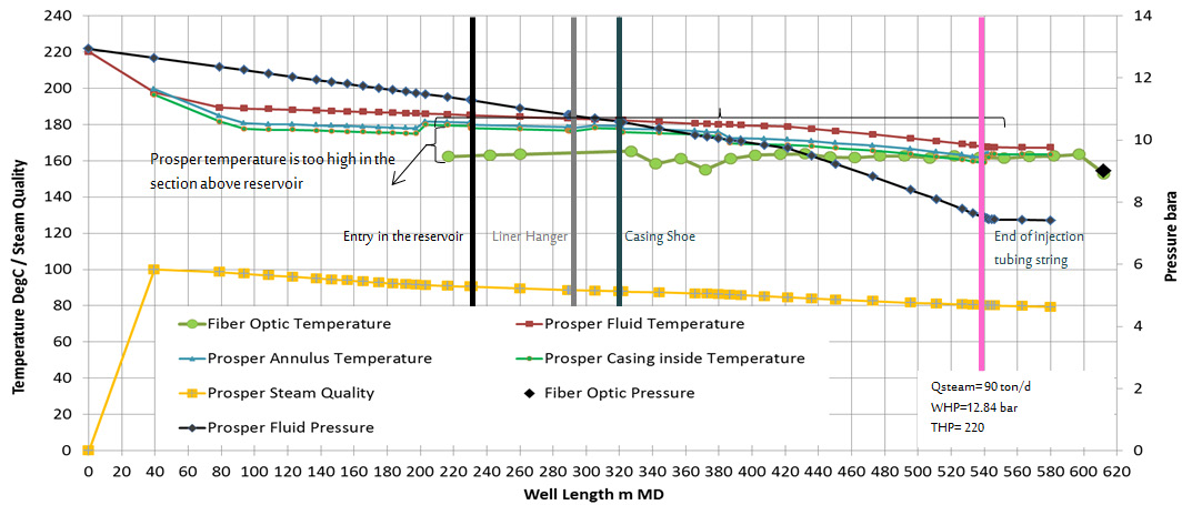
During injection through well #1 (Figures 8 through 14), the temperature is uniform along the slotted liner. It appears that the well shoe remains warmer than the rest of the well section, even when the well is shut down. This corresponds also to the Panonien sand section, after the long section of carbonate. Furthermore, the steam is not injected uniformly in the reservoir, but rather to zones with least resistivity (good rock properties & good fluid mobility: either warm zone, or zone with gas), or/and closer to the end of the injection string. With increase of gas production, the temperature profile does not change and the gas could also come from this most productive area. With high water cut, the temperatures in the middle well section are smaller than with lower water cut. It is not possible to see where the water corresponding to the increasing water cut is coming from – most likely also from the most productive zone, i.e. the well toe. During steam injection, the measured temperature and pressure do not correspond to the saturation conditions – big concerns that only hot water is injected. To get to the saturations conditions, the pressure should be ~2bar lower, could it be measurement error (~22% error)? Could the pressure gauge be disrupted by high temperatures? Prosper model could not reproduce those measurements. For the given injection conditions it would predict a ~80% steam quality. During steam injection in well #1, the temperatures are uniform in the slotted liner. It seems that more steam goes into reservoir sections with least resistivity and close to the end of the injection tubing string. The following points are extracted based on the results:
- The location of the end of the injection tubing string has an effect
- Preliminary Prosper models would predict: steam quality ~80% - 60% to tubing shoe for injection rate 90- 50 t/d
- Differences between measured wellhead temperature in time of injection phase and FO sensor temperature are around 40 -50°C
- Differences between measured wellhead pressure and FO sensor pressure are around 3-4 bar in CSS time
- Measurements in well #1 during steam injection did not correspond to saturation conditions, which should indicate hot water injection only
- This is the reason why Prosper model needs improvements regarding the pressure and temperature measurement error margin or further investigations over reservoir parameters
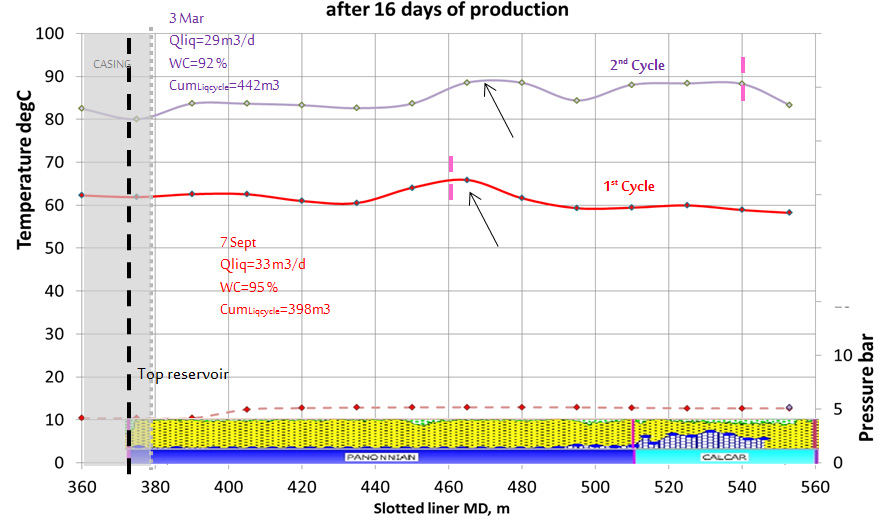
- It’s hard to qualitatively assess what is happening toward the well heel. The measured temperature may reflect more the well flow from the other well section, than the inflow from the reservoir; 1. Other pressure sensors are required apart from toe (i.e. to heel ); 2. Need of the permanent electrical power source to avoid wrong readings after electrical breaks Another steam injected well called well # 2 is also studied as shown from Figures 16 through 23. The temperature profile after 16 days of production for the 2 cycles is different (Figure 16). This could indicate that the location of the injection tubing string had an effect. It seems that injecting where mud losses where encountered helped cleaning this part of the well, as the temperatures in this zone are higher than in the previous cycle. After 29 days of production (Figure 17), both cycles showed a hot producing zone at ~460m MD. For the 2nd cycle the cold zone at 480-490m MD can be seen, but then the well is relatively warmer toward the toe, which could confirm its contribution – except for the last sensor that records smaller temperature. However, the difference in the temperature profile of the 2 cycles toward the well toe is confirmed over the next five periods: 39, 60, 90, 120, and 150 days (Figures 18 through 22). Moreover, another model was built using Prosper software to predict well temperatures and pressures along the wellbore profile, then compare with the FO measurements for well # 2. Figure 23 show a slightly match between Prosper model and FO data measured. However, there are still lots of things to sort in Prosper, but for this rate, Petroleum Expert 5 correlation gives a reasonable result. The calculated steam quality is ~68%. The problem with Prosper is to match the range of rates with the same correlation. This could not be achieved. During injection in well # 2, the temperatures are uniform along the well during steam injection. However having the steam in the slotted liner during injection, does not guaranty that the steam is injected uniformly along the well section. Changing the end of the injection tubing string location in the well had an effect in the temperature profile. It seems that for the 2nd cycle, the zone that had severe mud losses during drilling has been cleaned and has a better contribution. There is a zone at ~460m MD that remains warmer than the rest of the well – it corresponds to the end of the tubing string of the Aug 14 steam injection – but it can also be observed for the 2nd cycle. Either this zone is hot because it received directly a lot of steam in Aug14, i.e. this is due to the injection tubing string location Also, it has particularly good properties as shown in the well log, so it is easier for the steam to get into this zone. With time a colder zone can be observed from 480 to 490m MD. This is most likely aquifer water coning. Another one could be briefly observed at 430m MD, but seemed later masked either by fluid coming from the other well sections or because its contribution is small. The 1st well section [380, 381, 382, 383, 384, 385, 386, 387, 388, 389, 390, 391, 392, 393, 394, 395, 396, 397, 398, 399, 400, 401, 402, 403, 404, 405, 406, 407, 408, 409, 410, 411, 412, 413, 414, 415, 416, 417, 418, 419, 420, 421, 422, 423, 424, 425, 426, 427, 428, 429, 430] mMD where logs interpretation attributes good porosity does not seem to contribute much to production. A Prosper model would predict a 68% downhole steam quality during the February 15 steam injection.
Conclusions
In conclusion, the Suplacu field is served as a prototype for other fields of a similar kind in Romania and is a significant testing ground for cutting-edge heavy oil exploitation technology. The extraction of heavy crude oil at advanced maturity circumstances, when thermal processes and specialized pumps are necessary to sustain economic production, is shown by this reservoir. In heavy- oil fields like Suplacu, this study has demonstrated that real- time distributed fiber-optic sensing (FOS), which includes distributed temperature sensing (DTS) and distributed acoustic sensing (DAS), is a useful and effective method for improving SAGD performance monitoring. In order to accurately visualize the evolution of the steam front and identify injection irregularities, the field pilot showed that FOS systems can consistently record high-resolution thermal and acoustic data over the whole length of horizontal injector wells. Because it provides geographically and temporally rich information, this continuous monitoring technique performs noticeably better than conventional point-based sensors. More precise history matching and a better comprehension of reservoir behavior, including the identification of heterogeneities and steam channeling, were made possible by the integration of FOS data with a coupled wellbore- reservoir simulation model. The efficacy of the existing data infrastructure, which was shown to be reliable enough for prolonged monitoring periods, was also confirmed by the pilot. Despite early problems with sensor power failures and data synchronization, they were resolved later in the trial. The technical viability of applying FOS in established, onshore heavy-oil operations was generally validated by the field study. The system was useful not just for real-time monitoring but also for optimizing well performance during the SAGD cycle and guiding steam injection schemes.
Recommendations
Based on the results and discussions, the recommendations are divided into the main six items as following:
- Wider Deployment of FOS Systems: To provide complete temperature and flow profiling, assist cross-well diagnostics, and enhance compliance control, DTS and DAS systems should be installed across injector and producer wells.
- Improved Instrumentation: To further enhance coupled model calibration and improve pressure diagnostics, install pressure gauges at the wells’ toe and heel portions.
- Workflows for Automated Optimization: Use automated simulation-feedback loops with real-time FOS data to continually modify steam injection rates and identify operational irregularities early.
- Advanced Data Analytics: Use machine learning techniques to analyze and analyze vast amounts of auditory and thermal data, allowing for automatic anomaly identification (such as coning, steam breakthrough, or crossflow).
- Scalability Assessment: To evaluate the wider applicability and scalability of this integrated monitoring and modeling process, conduct further pilots in other Suplacu field regions and in heavy-oil reservoirs with comparable geology.
- Increase Power and Data Redundancy: Reduce the possibility of data gaps during crucial injection or production stages by increasing system power redundancy and communication dependability. This will guarantee continuous data collecting. Operators may considerably enhance reservoir management, lessen their impact on the environment by using steam more efficiently, and increase the productive life of heavy-oil assets by integrating high-resolution sensor technologies with dynamic simulation and optimization.
References
-
Lake LW (1989) Enhanced oil recovery, I: Fundamentals and analyses. Volume 17A, Elsevier.
-
van Poolen KH, Associates Inc. (1980) Fundamentals of enhanced oil recovery. PennWell Books.
-
Smolen J (2015) Fiber Optic Sensors for Well and Reservoir Monitoring. Gulf Publishing.
-
Li Q (2021) Advances in distributed fiber optic sensing in thermal EOR applications. Energy Reports 7: 1489- 1505.
-
Maldonado F (2012) Thermal monitoring of SAGD wells using DTS. J Canadian Petroleum Technology 51(2): SPE- 146994.
-
Mateeva A, Lopez J, Potters H, Mestayer J, Cox B, et al. (2014) Distributed acoustic sensing for reservoir monitoring with vertical seismic profiling. The Leading Edge 33(7): 936-943.
-
Farhadiroushan M (2019) Integrated DAS/DTS monitoring for heavy oil steam injection. First Break 37(6): 89-94.
-
Hollaender F (2013) Distributed temperature and strain sensing for reservoir monitoring. SPE Journal 18(5): 1004-1015.
-
Ghani A (2019) Optimizing SAGD performance using DTS data. SPE Heavy Oil Conference, SPE-195510.
-
Bukhamsin A (2017) Optimizing cyclic steam stimulation using real-time DTS. Journal of Petroleum Science and Engineering 149: 778-788.
-
Harrison S (2016) Thermal front tracking in in-situ combustion using DTS. In Proc. SPE Improved Oil Recovery Conference, SPE-179661.
-
Zhang W (2019) High-temperature fiber optic sensors for steam flooding monitoring. Sensors 19(17): 3748.
-
Fidanboylu K (2019) Challenges in high-temperature fiber optic sensors. Journal of Sensors 2019: 1-15.
-
Jiang H (2020) Machine learning applications for DTS data interpretation in SAGD. SPE Journal 25(4): 2123- 2137.
-
Sani M (2022) Machine learning-driven interpretation of DTS data in SAGD. SPE Journal 27(2): 732-743.
-
Martins J (2022) Hybrid DAS/DTS monitoring for SAGD optimization. Sensors 22(5): 1922.
-
Okonkwo C (2023) 4D reservoir monitoring using fiber optic sensors. SPE Reservoir Evaluation & Engineering 26(1): 123-135.
-
Zhao X (2021) Data analytics for DTS in heavy oil fields. IEEE Access 9: 155783-155794.
-
Culshaw B (2005) Optical fiber sensor technologies: opportunities and—perhaps—pitfalls. Journal of Lightwave Technology 22(1): 39-50.
-
Measures RM (2006) Structural Monitoring with Fiber Optic Technology. Academic Press.
-
Kersey AD (2007) A review of recent developments in fiber optic sensor technology. Optical Fiber Technology 9(3): 269-287.
-
Rao YJ (2008) Recent developments in fiber optic sensors for aerospace applications. Sensors and Actuators A: Physical 149(1): 21-29.
-
Bao X, Chen L (2010) Recent progress in distributed fiber optic sensors. Sensors 10(3): 1898-1917.
-
Hartog AH (2011) An Introduction to Distributed Optical Fibre Sensors. CRC Press.
-
Soto MA (2012) Real-time monitoring of temperature in geothermal reservoirs with DTS. Geothermics 41: 9-16.
-
Masoudi A, Newson TP (2013) Distributed optical fibre dynamic strain sensing. Sensors 13(9): 11782-11813.
-
Liehr S (2014) Novel optical frequency domain reflectometry for distributed sensing. Optics Express 22(7): 8124-8134.
-
Froggatt ME, Moore J (2015) High-spatial-resolution distributed strain and temperature sensing using Rayleigh scatter in optical fiber. Applied Optics 54(9): 2180-2186.
-
Zhan Y (2016) Multiplexed fiber optic strain sensors for structural health monitoring. Optics Letters 41(3): 575- 578.
-
Parker TR (2017) Distributed acoustic sensing for seismic applications. Nature Communications 8(1): 1-9.
-
Selker JS (2018) Environmental sensing by DTS: hydrology and beyond. Water Resources Research 54(10): 7391-7401.
-
Zhang X (2019) Integrated fiber optic pressure and temperature sensors. Sensors and Actuators A: Physical 287: 12–19.
-
Fidanboylu K, Efendioglu HS (2020) Fiber optic sensors: novel materials and fabrication methods. Sensors 20(10): 2971.
-
Farhadiroushan M (2021) DAS for monitoring CO₂ storage. International Journal of Greenhouse Gas Control 110: 103452.
-
Smith JA, Farahi F (2022) Hybrid optical fiber sensing with FBG and Raman scattering. Journal of Sensors 2022: 1-12.
-
Wang Y (2023) Machine learning-enhanced distributed fiber optic sensing data analysis. Journal of Lightwave Technology 41(5): 1433-1442.
-
Xu H (2024) Ultrafast optical fiber sensing for railway infrastructure. IEEE Sensors Journal 24(2): 234-240.
-
Huang J (2025) High spatial resolution distributed sensing with photonic crystal fibers. Optics Letters 50(3): 312-315.
-
Branoui G, Dinu F, Stoicescu M, Ghețiu J, Stoianovici D (2021) Half a century of continuous oil production by in-situ combustion in Romania – Case study Suplacu de Barcau field. MATEC Web of Conferences 343: 09009.
- Nigeria’s Vulnerability in the Face of Global Energy Policy
- A Simulation Study of Investigation of Optimum Oil Production Performance by Applying Various Gas Injection Methods in Oil Reservoir
- Characterization of Permo-Triassic Reservoirs through Thermal Maturity Assessment of Westphalian Source Rocks in the Cheshire Basin
- Influence of Microwax on the Rheological and Thermal Behaviour of a Wax Crude Oil
- Rapid On-Site Determination of the Total Petroleum Hydrocarbon Content of Soils by Handheld Fourier Transform Near-Infrared Spectroscopy: Development of a Global, Site- and Scanner- Independent Calibration Model
- Isothermic, Kinetic and Thermodynamic Studies of Chromium (VI) Ions Adsorption on Composite Adsorbent of Chitosan- Eggshell Activated Carbon