CFD Simulation of a Crude Oil Transport Pipeline: Effect of Water
In the present study, a 3D two-phase CFD simulation has been performed to investigate crude oil-water core annular flow through a crude oil transport pipeline in a real scale with 100 mm diameter and 1000 m length. Results of pressure profile and volumetric fraction distribution of the crude oil and water phases are analyzed. It was verified that the heavy oil core surrounded by a water film flowing in the pipeline considerably decreases pressure drop in the crude oil transportation pipeline and therefore reduces the pumping power consumption (about 50%). The results revealed the water film is formed near the pipe wall at the beginning of the flow but this annular pattern does not remain until the end of the pipe and is destroyed after about 4 meters from the pipe inlet.
Introduction
The petroleum is the most important sources in the world energy sector. Over the past decades, high demands for oil products and therefore increase in crude oil extraction have led to depletion of light oil reserves. Nowadays in the world a great number of oil reserves are heavy type. Crude oil is often extracted from remote locations away from refining plants. Generally crude oil has been transported via pipelines. Due to its unfavorable characteristics (high viscosity), the transport of heavy crude oil is complex, costly and requires a large amount of power to pump it. In recent years, different methods have been proposed to solve this problem such as heating the crude oil (with electrical heating or the injection of a heated fluid), using steam to forming oil-in-water emulsions, injection of light oil or other additives, and using water-lubricated transport or core annular flow [1, 2, 3]. The core annular flow is a technique to form a water film in the pipe that surrounds the oil. The presence of water film avoids contact of crude oil with the pipe walls and therefore reduces the pressure drop by friction.
Previous studies have investigated crude oil transportation using the core annular flow technique. They have reported the core annular flow is an effective method that can be used in pipelines to transport heavy crude oils [4, 5, 6, 7, 8, 9].
The hydrodynamics of two phase (oil-water) core annular flow is substantially complex as there are interaction between the phases and between any individual phase and the pipe wall. In the recent years, Computational Fluid Dynamics (CFD) has become a robust tool for modeling oil-water multiphase flows. CFD is a branch of fluid mechanics that predicts flow hydrodynamics by numerical solving the governing equations. Several researchers have studied oil-water core annular flows in different pipes (curved, vertical, horizontal) and fittings (bend, tee, etc.) using CFD [1,2,10- 15 ]. Previous studies have covered many aspects of oil- water core annular flows. However their simulations have been performed for the short length not in real scale. Therefore the aim of this study is to simulate a pipeline in the real scale and evaluating effect of core annual flow on total pressure drop of the crude oil pipeline.
Geometry and Mesh Generation
In this numerical simulation, 3D geometry was used. The simulated pipeline was a horizontal carbon steel pipe with 100 mm diameter and 1000 m length. A crude oil core flow with 80 mm diameter and a water film with 10 mm depth were considered in the pipe. Figure 1 sketches the computational domain for this pipeline.
Geometry and grid were consolidated using GAMBIT2.4.6 software. Structured meshing with hexahedral elements was implemented near the pipe wall since a thin water film is expected here. Therefore, a 3D grid with 177450 hexahedral elements was generated for each 10 m of pipeline (computational domain). A chunk of the generated mesh used in the present study is depicted in Figure 2.
Mathematical Modelling and Governing Equations
In this study, the two-phase Volume of Fluid (VOF) approach was used for modelling the crude oil-water core annular flow in the pipeline. This approach models two immiscible fluids (oil and water) by solving a single set of momentum equations and tracking the volume fraction of each of the fluids throughout the computational domain. The following mass and momentum conservation equations are implemented in the VOF model [2, 12, 16]. The continuity and α-equation for phase q:
$$ \mathrm {E} = \mathrm {E} _ {1} + \mathrm {E} _ {2} + \dots + \mathrm {E} _ {n} $$ pq qp q p m m ( ) .( u ) t ( ) s αρ αρ $$ \frac {\partial \left(\alpha_ {\mathrm {q}} \rho_ {\mathrm {q}}\right)}{\partial \mathrm {t}} + \nabla . \left(\alpha_ {\mathrm {q}} \rho_ {\mathrm {q}} \vec {\mathrm {u}} _ {\mathrm {q}}\right) = \sum_ {\mathrm {p} = 1} ^ {\mathrm {n}} \left(\dot {\mathrm {m p q}} - \dot {\mathrm {m q p}}\right) + s $$ n $$ \mathrm {E} = \frac {1}{2} \mathrm {A} ^ {2} + \mathrm {B} ^ {2} $$ q q (1) q q q n $$ \sum_ {\mathrm {p} = I} ^ {\mathrm {n}} \alpha_ {\mathrm {q}} = $$ (2) 1 1 q p Where 𝑢𝑞 ⃗⃗⃗⃗ , ρq, Sq and αq are velocity, density, mass source term and volume fraction of phase q, respectively. 𝑚̇ 𝑝𝑞and𝑚̇ 𝑞𝑝 characterize mass transfer between pth and qth phases. The momentum equation: A single momentum equation is solved throughout the domain, and the resulting velocity field is shared among the phases.
𝜕 𝜕𝑡(𝜌𝑢⃗ ) + ∇. (𝜌𝑢⃗ 𝑢⃗ )
(3) = −∇𝑝+ ∇. [𝜇(∇𝑢⃗ + ∇𝑢⃗ 𝑇] + 𝜌𝑔 + 𝐹
Where ρ,𝑢⃗ ,p, µ, 𝑔 and 𝐹 are density, velocity, pressure, viscosity, gravitational acceleration and body force, respectively.
Physical Properties of Fluids and Boundary Conditions
Table 1 lists the considered characteristics of the crude oil and water [17].
| Crude Oil | Water | |
|---|---|---|
| T (°C) | 25 | 25 |
| μ(Pa.s) | 2 | 0.001 |
| ρ (kg/m3) | 863.5 | 998 |
| oil-water interfacial tension (N/m) | 0.022 |
Table 1: Considered physical properties of the crude oil and water.
| Item | Boundary Condition | ||||
|---|---|---|---|---|---|
| inlet | water velocity inlet (40 mm ≤ r ≤ 50 mm)= 2 m/s | ||||
| crude oil velocity inlet (r < 40 mm)= 2 m/s | |||||
| outlet | out flow | ||||
| Pipe wall | non-slip wall |
Simulation Procedure
Using ANSYS Fluent18.1, the finite volume method was implemented to discretize the differential equations of continuity and multiphase flow (VOF) in the computational domain. To calculate the pressure field, the Coupled algorithm was used for coupling pressure and velocity equations for the two phases. The Coupled algorithm solves the momentum and pressure-based continuity equations together. The PRESTO! and second order upwind scheme were applied for interpolation of the field variable from cell centers to faces of the control volumes. The convergence criteria were set at 10-3. The numerical simulation was run with an Intel® Core i5 CPU (2.2 GHz) and 4GB RAM; the results were converged after 6600 iterations and the run time was about 9.5 hr.
Results and Discussion
Volume Fraction Field
Figure 3 shows the volume fraction of oil phase in the pipeline. The results reveal that the water film is formed near the pipe wall at the beginning of the flow but this annular pattern does not remain until the end of the pipe. Figure 4 shows the volume fraction of water phase in the cross section of pipe at different distance from the pipe inlet. This figure shows the presence of water film near the pipe walls. However, the annular flow pattern is destroyed after about 4 meters from the pipe inlet. This is because the oil phase is less dense than the water phase and tends to concentrate in the upper part of the pipeline.
Pressure Field
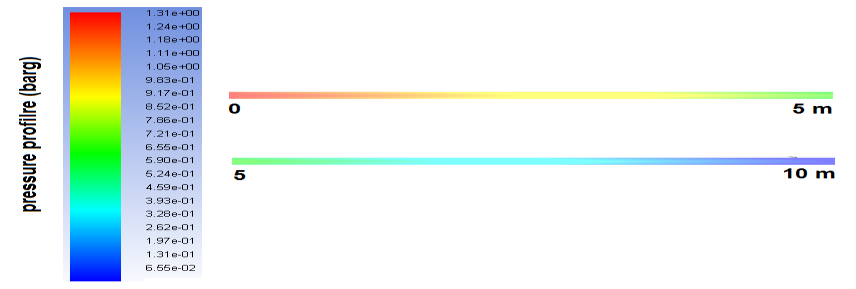
In order to evaluate the effect of core annular flow on the pressure profile of pipeline, the CFD modeling was repeated in the case of single phase crude oil flow. The pressure profile for single phase flow in the pipeline (with 10 m length) is shown in Figure 5.
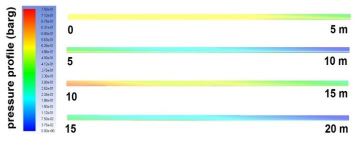
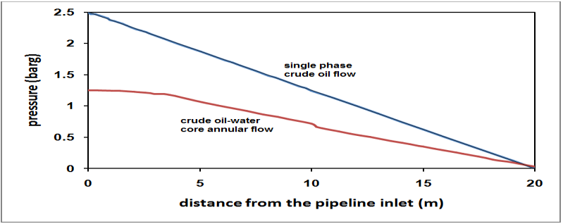
Comparison of pressure drops in the pipeline (with 20 m length) for two cases of single (crude oil) phase and core annular flow is depicted in Figure 7. The results illustrate a lower pressure drop in the pipeline for oil- water core annular flow, especially in the region that the annular flow pattern is not destroyed yet (up to about 4 m). Figure 7 shows using core annular flow technique reduces contact of crude oil with the pipe walls and therefore decreases pressure drop in the crude oil transportation pipeline significantly (about 50%).
Energy Efficiency
According the pumping power that is needed to transportation of crude oil through the pipeline, the efficiency of core annular flow technique can be evaluated. Table 3 summarizes the required pumping power for crude oil transportation with and without using the core annular flow technique.
| Single (crude oil) phase flow | Water-oil core annular flow | |
|---|---|---|
| Pressure drop in the pipeline (0 to 10 m) | 1.31 bar | 0.57 bar |
| Pressure drop in the pipeline (10 to 20 m) | 1.31 bar | 0.68 bar |
| Pressure drop in the pipeline (20 to 1000 m) | 128.38 bar | 66.64 bar |
| Total pressure drop in the pipeline | 131 bar | 67.89 bar |
| Flow rate | 56.52 m3/hr | 56.52 m3/hr |
| Required pumping power (electrical) | 457 kW | 236.9 kW |
| Electrical power consumption in a year | 4003709 kWh | 2074899 kWh |
Table 3: The required pumping power for crude oil transportation.
According to the pumping power calculation, using core annular flow technique can lead to about 50% reduction in the pipeline pressure drop and pumping power consumption.
Conclusions
According to the results of CFD simulation of crude oil- water annular flow in a pipeline, the conclusions are summarized as follows:
- The water film is formed near the pipe wall at the beginning of the flow but this annular pattern does not remain until the end of the pipe and is destroyed after about 4 meters from the pipe inlet.
- Using core annular flow technique reduces contact of crude oil with the pipe walls and therefore decreases pressure drop in the crude oil transportation pipeline significantly (about 50%).
- There is a significant decrease (about 50%) in the pumping power consumption for crude oil transport through the pipeline proving the efficiency of the heavy oils transportation using the core annular flow technique.
However it must be noted that the effects of other factors such as crude oil rheological properties, the actual route and slope of pipeline can be investigated to make more accurate analysis of the two-phase flow and get more precise results. These studies can be a base for the future research in this area.
References
-
Conceição S, Lima A, AndradeT, NetoS, OliveiraV, et al. (2017) Applying CFD in the Analysis of Heavy-Oil Transportation in Curved Pipes Using Core-Flow Technique. Int J of Multiphysics 11(2): 169-184.
-
Al Jadidi S (2017) Lubricated Transport of Heavy Oil Investigated by CFD. University of Leicester, UK.
-
Saniere A, Hénaut I, Argillier JF (2004) Pipeline Transportation of Heavy Oils, a Strategic, Economic and Technological Challenge. Oil & Gas Science and Technology 59(5): 455-466.
-
Bai R, Chen K, Joseph DD (1992) Lubricated pipelining: stability of core-annular flow. Part 5. Experiments and comparison with theory. Journal of Fluid Mechanics 240: 97-132.
-
Bannwart AC (2001) Modelling aspects of oil-water core annular flows. Journal of Petroleum Science and Engineering 32(2-4): 127-143.
-
Bensakhria A, Peysson Y, Antonini G (2004) Experimental study of the pipeline lubrication for heavy oil transport. Oil & Gas Science and Technology 59(5): 523-533.
-
Ghosal S (1996) An analysis of numerical errors in large-eddy simulations of turbulence. Journal of Computational Physics 125(1): 187-206.
-
Joon Sang L, Xiaofeng Xu, Richard H (2004) Large eddy simulation of heated vertical annular pipe flow in fully developed turbulent mixed convection. International Journal of Heat and Mass Transfer 47(3): 437-446.
-
Lovick J, Angeli P (2004) Experimental studies on the dual continuous flow pattern in oil-water flow. International Journal of Multiphase Flow 30(2): 139- 157.
-
Gupta R, Turangan CK, Manica R (2016) Oil‐water core‐annular flow in vertical pipes: A CFD study. The Canadian journal of Chemical Engineering 94(5): 980- 987.
-
Dehkordi PB, Colombo LPM, Guilizzoni M, Sotgia G (2017) CFD simulation with experimental validation of oil-water core-annular flows through Venturi and Nozzle flow meters. Journal of Petroleum Science and Engineering 149: 540-552.
-
Kaushik VVR, Ghosh S, Das G, Kumar Das P (2012) CFD simulation of core annular flow through sudden contraction and expansion. Journal of Petroleum Science and Engineering 86–87: 153-164.
-
Jiang F, Wang Y, Ou J, Xiao Z (2014) Numerical Simulation on Oil–Water Annular Flow through the Π Bend. Ind Eng Chem Res 53(19): 8235-8244.
-
Ghosh S, Das G, Das PK (2010) Simulation of core annular down flow through CFD- a comprehensive study. Chem Eng Process 49(11): 1222-1228.
-
Sumana G, Das G, Das PK (2011) Simulation of core annular in return bends-A comprehensive CFD study. Chem Eng Res Des 89(11): 2244-2253.
-
ANSYS Fluent 18.1 Theory Guide (2017) ANSYS Inc.
-
Niazi S, Mirarab Razi M, Hashemabadi SH (2014) CFD Simulation of Acoustic Cavitation in A Crude Oil Upgrading Sonoreactor and Prediction of Collapse Temperature and Pressure of A Cavitation Bubble. Journal of Chemical Engineering Research and Design 92(1): 166-173.
- Nigeria’s Vulnerability in the Face of Global Energy Policy
- A Simulation Study of Investigation of Optimum Oil Production Performance by Applying Various Gas Injection Methods in Oil Reservoir
- Characterization of Permo-Triassic Reservoirs through Thermal Maturity Assessment of Westphalian Source Rocks in the Cheshire Basin
- Influence of Microwax on the Rheological and Thermal Behaviour of a Wax Crude Oil
- Real-Time Monitoring and Performance Optimization of Steam Injection in Heavy Oil Reservoirs Using Fiber Optic Sensing and Integrated Predictive Simulation Models
- Rapid On-Site Determination of the Total Petroleum Hydrocarbon Content of Soils by Handheld Fourier Transform Near-Infrared Spectroscopy: Development of a Global, Site- and Scanner- Independent Calibration Model