The Impact of Marine Environment on Jackup Rig Stability
Changing the conditions of offshore environment influences the offshore units' stability. In paper, a study of the impact of marine environment on a jackup rig was implemented. Firstly, the procedures of departure, transit, and emplacement on any emergency jacking location / stand by location are reviewed. After that, the conditions of weather forecasting are predicted and computed such as wave and wind lengths, speeds, and heights. Maps of changing wind and wave conditions are plotted. Surveying methods are used to determine the final location of the jackup rig. Maps of positioning the jackup rig are constructed. Additionally, the impact forces on the rig derrick are therefore computed. The developed results are effectively predicting the safe conditions and optimizing the positioning survey of the rig.
Introduction
The choices to use a jackup rig would also be affected by the same variables, but the jackup would usually be strongly favoured by a smaller number of wells and shallow water. The platform design should provide enough space for the jackup to be placed across the platform without damaging it. In order to ensure the functionality of the two, this will enable the operator to look at a specific rig and sign a contract for this rig. With tugs and work boats, the rig will be spotted close to the platform. The anchor mechanism for the rig would be put out and the tugs would help locate the rig over the deck. The anchor pattern of the rig should ensure adequate holding power and not interact with the platform’s daily operations, such as pipelines, crew and work vessels, etc. To decrease the anchor-handling issue, anchor piles are often mounted on the platform. The jackup is the most stable of all drilling units when elevated, and drilling from a jackup is like drilling on shore. In water depths of more than 50 ft, the jackup is the least expensive type of rig to install and run. The depth limit for water is around 350 ft. Because of their hull form, jackups have poor mobility that makes them hard to tow, and many tugs may be required to sustain a speed of
With the spud cans fully full, the platform is believed to be afloat. The operating guidelines and preparatory to go-on- location after initial check list have been performed correctly. Jacking processes are important and it is important to meet the following conditions [1, 2, 3, 4, 5]:
- Ensure that good weather prevails during this operation and that the roll and pitch of the platform does not exceed the limits defined on the platform design curves.
- It is suggested that the platform be attached to the bottom and raised only during daytime hours.
- Barriers that could damage the spud cans should be removed from the ocean floor.
- Lower the legs in series to provide enough time for generator recovery before starting the lowering of the next leg. If it is about 10 to 15 feet above the bottom, stop each leg.
- To reduce swing and/or drift, check the wind, wave, and current direction and align the platform with tugs and anchors.
- Lower the legs to the bottom of the ocean and proceed to lift the platform to the ideal preload height, keeping the level of the platform during elevation within 0.3 of one degree. Do not permit the distance between the wave crest and the bottom of the hull to be less than 5 feet when elevated.
- Pre-loading a. If the variable load on board is lower than the maximum allowable, the amount of load needed to simulate the maximum allowable variable load shall be determined and the preload tanks shall be filled with this quantity of seawater distributed equally on both legs. b. Load all legs consistently with the defined amount of preload, ensuring an even load on all legs. By changing the rate of preload flow or, if required, by lowering the high corner of the platform, sustain the platform level to within 0.3 of one degree.
- Continue reloading until all settling has occurred and the platform is stabilized.
- Discharge all pre-loading.
- Uplift the platform to the optimal drilling height, keeping the level of the platform at all times within 0.3 of one degree.
- Switch the console master key to OFF position when the elevation is achieved.
The casualties from jackups fell into the following categories [1, 2, 3, 4, 5]:
- Undertow 36%.
- Moving on/off = 27%.
- Blowouts 27%.
- Severe storms = 10%.
Offshore Rig Design Rules of Thumb
Rules of thumb [2] which are recommended to be taken in designing an offshore rig are
- Potable-water requirements 65 gal per person per day
- Living quarters 50 sq ft per person
- Engine-generator deck area 10 kW/sq ft
- Motor deck area 60 hp/sq ft
- Engine deck area 16 hp/sq ft
- Engine-generator deck load 260 lb/sq ft
- Motor deck load 440 lb/sq ft
- Engine deck load 170 lb/sq ft
- Engine-generator weight 291b/Kw
Offshore Units Stability
A stability is the ability of an offshore unit to remain afloat. The stability is classified into two types: intact stability and damaged stability. For every rig, the designer or engineer should provide the rig owner with a Stability Booklet which should contain [3]: a. Hydrostatic Properties b. Cross Curves of Stability c. Statical Stability Curves d. Dynamic Stability Curves.
Items (c) and (d) should be sufficient to cover the normal operating range of the vessel. In order to understand the above terms, a description of each item should be presented as follows [3]: a. Hydrostatic Properties are constructed from the shape of the underwater portion of the rig and can be utilized to estimate the rig weight and the location of the centroid, longitudinally and transversely. It has several other benefits, however the most often one is when moving a rig. b. Cross Curves of Stability are also generated from the underwater portion of the rig and are used by the designer to determine the amount of stability the vessel when it is not in the upright position. c. Statically Stability Curves are developed from the cross curves of stability and are curves of righting arm. They are sometimes referred to as GZ curves. d. Dynamic Stability Curves are produced from the statically stability curves and determination of the overturning moment caused by a wind of a given velocity. This curve is probably the most important of all curves because it illustrates whether or not the rig can be towed during the forecasted weather, while remaining within the safety parameters of the regulatory bodies. e. Allowable Dynamic Stability KG Curves are generated from the dynamic stability calculations. These curves are a growth of the dynamic stability curves_,_ and they simplify the rig mover’s job by eliminating the need to prepare a calculation of dynamic stability every time he decides on a possible tow condition. f. Damaged Stability Calculations should be prepared for the effect of damage to the outside compartments or flooding into any compartment. These calculations should show that the vessel has sufficient reserve stability to survive either damage or flooding. If the ABS “Rules for Building and Classing Offshore Mobile Drilling Units 1973” are applied to the vessel, the ability to survive damage or flooding must be considered in association with the over~ turning effect of a 50-knot wind [4, 5]. g. Motion Response Analysis is the study of the rig in a “hove to” state. This is the position when “going on location,” and the results of this analysis are used to determine the stresses induced when a jack-up leg touches bottom or those caused by mooring forces on a drillship or semisubmersible. h. Lightship Characteristics are probably the most used (or misused) information that should be supplied. This information is prepared either from a series of accurate weight calculations or from an inclining experiment, or both. The calculations determine the weight and centre of gravity in all directions of the dry rig, i.e., no variables of any kind are included.
Wind, Wave, and Current Forces on Offshore Structures
The primary design loads on mobile drilling units and other offshore structures are the forces produced by wind, wave, and current. These forces are dynamic and ever- changing; they can seldom be expressed as a mathematical function of time. They are statistical in nature and should be handled by means of statistical tools. In order to evaluate wave loads on an offshore structure, the most commonly method which is based the calculations on one or more design waves of specified height and period. Furthermore, for estimating the wave loads on fixed and floating offshore structures, two methods normally utilized and their characteristic features are [3]:
- Spectral Analysis Method. It is used for floating structures mainly, but also fixed structures provided that the nonlinear loads are small compared to the linear loads (large diameter columns). . Linear statistical analysis. Also, it helps to evaluate of the most probable largest wave loads that will occur during the structure’s lifetime.
- Design Wave Method. It is used for both fixed and floating offshore structures. It also helps to design wave of specified height and period. Moreover, evaluation of the loads resulting from a regular wave with height and period as specified can be determined.
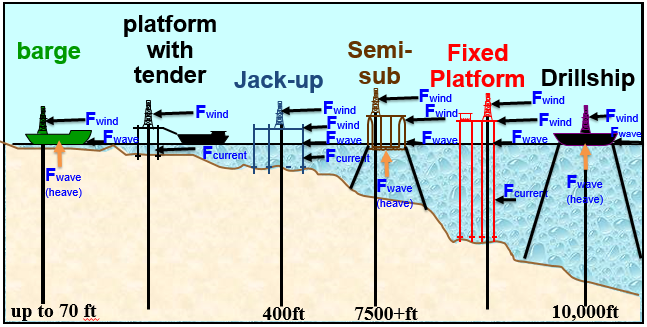
Applying the design wave method, the combined effects of wind, waves, and current on a fixed offshore structure are normally treated as quasi-static forces. This is valid in most cases, particularly if care is taken in determining the “worst case” loading. The environmental loads acting on different drilling units are simplified in Figure 1.
Wind
Wind velocity is an important parameter in wind forces. Normally, two different wind velocities are specified in the design criteria for offshore structures, the N year sustained and the N year gust wind velocity. These are defined as follows [3]:
- N Year Sustained Wind Velocity. This is the average wind velocity during a time interval (sampling time) of one (1) minute with a recurrence period of N years.
- N Year Gust Wind Velocity. This is the average wind velocity during a time interval (sampling time) of three (3) seconds with a recurrence period of N years.
Velocity Variation with Height above Sea Surface [3]: The sustained wind velocity is often considered to vary with height above sea surface according to the following formulas [6]:
1
10 10 z V V z τ =
(1) Davenport has proposed a value of t= 7 for open country, flat coastal belts, and small islands situated in large areas of water. The following formula, adopted as basis for the DnV Rules [4, 5], is a compromise between the one-seventh power law (Equation 1) and Davenport’s conclusion:
0.93 0.007 10 V V Z z = + (2)
According to the DnV Rules [4, 5], the gust velocity is not to be taken less than:
( ) 1.53 0.003 10 G V V Z z = + (3)
Wind Forces of Individual Members [3]: Wind forces increases with the square of the wind velocity and in direct proportion to the exposed area. There are other factors that affect the wind forces such as the shape of the exposed areas and their height above sea level. Based on the one-seventh power law, the wind forces can be expressed as follows:
2 0.00388 (Theunitsareimperial) 10 W F C CV A H − = (4)
The height coefficient CH may be expressed as:
27 H C , in 30 z Z is ft =
(5) The shape coefficient C varies from 0.5 for cylindrical shapes to 1.5 for structural steel shapes.
The force acting on the area A in the direction of the wind then becomes:
3 1 2 0.00388 10 y H F C CV ASin α − = (6)
The formula generally accepted at DnV [4, 5] for calculating wind forces is:
2 z W V F C Sin A Theunits aremetric α = (7)
1 ,( ) 16 The force acting on an area A in the direction of the wind then becomes:
2 z W V F C Sin A α = (8)
1 16
![Figure 2: Two different methods for decomposing wind or drag forces: a. Decomposing velocity first, b. DnV approach [3].](/fulltextimages/6205/fig_2.png)
Figure 2 shows two formulae, differ by sin α1, which are used to determine the wind forces on offshore structure. For shape coefficient determination, the shape coefficient for short individual members (3-dimensional flow), according to the DnV Rules [4, 5] is to be taken as:
C C 0.5 0.1 , 5 L L d d = + < ∞
(9) The shape coefficient , can be determined according to the DnV Rules [4, 5]: 2 for flat bars, rolled section, and plate girders, 1.5 for rectangular sections, 0.7 for smooth circular of diameter >= 0.3 m, and 1.2 for cylindrical member of diameter < 0.3 m.
Current
Current forces are often considered in connection with wave force by adding vectorially the water particle velocities due to wave and current. Current velocity is regularly divided into two parts: wind induced current due to wind shear and tide-induced current. The variation of current velocity with distance above bottom is described as follows [3]:
17
1 1 cy w T y y V V V H H = +
(10) In open areas, the wind induced current of the still water level can be estimated as follows:
0.01 10 V V w = (11)
Where Vcy= Current velocity y m. above bottom, m/sec VT= Tide-induced current in the sea surface, m/sec Vw= Wind-induced velocity in the sea surface, m/sec H1= Water depth, m y= m. Above bottom V10= Sustained wind speed, m/sec
Waves
As mentioned earlier, there are two various methods used in evaluating the wave forces on fixed and floating offshore structures: spectral analysis method and design wave method [3].
Spectral Analysis Method Regular Waves: A regular deep water wave is approximately sinusoidal and its relationship between wave length and wave period can be described as follows (metric units):
2 2 g 1.56 2 T T λ π = = (12)
The maximum height for a regular wave is expressed as follows:
max 1 7 H λ = (13)
The responses of the regular waves can be described very well by linear functions of wave height, these responses can be represented by transfer functions.
Irregular Waves: In order to obtain a realistic description of the sea, irregular waves must be considered. However, these waves are more difficult to describe than the regular ones because the wave pattern never repeats itself. Although statistical methods may be used to describe the sea, they are not less exact. For describing irregular waves, it is necessary to distinguish between stationary conditions during a short time (= hours) and variable conditions during a long time (=months or years). In order to simulate waves mathematically by a wave spectrum, the following equations are taken into consideration [3]:
Stationary Conditions: Short term statistics [3]
( ) ( ) ( ) 2 2 , S S f w w ω α ω α = (14)
( ) 2 5 4 1 1 exp 2 2 2 2 8
− − = −
S T T w ω ω ω π π π π (15)
H T
13
2 2 f Cos α α π = (16)
( ) ( ) Y a Cos ti li li li li δ ω ξ = + (17)
( ) ( ) 2 2 1 2 i R i i i d S d Y a ω ω ω = ∑ (18)
( ) ( ) 2 2 2 R B S Y S ω ω = for constant Y within i ω ∆ wave forces on fixed offshore structures [3, 4, 5, 6, 7].
• Long Slender Elements ( Morison equation)
1 2 2 1 1 2 4 F gC LDV Sin gC D LV Sin w D M π ξ α ξ β = ∆ + ∆ (29) Where the drag coefficient CD ranges from 0.7 for circular cylinder to 1.5 for structure steel shapes, and the added mass coefficient Cm=CM-1 ranges from 1.0 for circular cylinders to 2 for structural steel shapes • Large Volume Structures A large body (e.g., oil storage tank) will reflect the waves producing disturbances to the velocity and acceleration field. The forces can be calculated by applying the Morison’s equation and diffraction theory Wave Spectra: The Pierson-Moskowitz spectrum [7] proposed the most generally wave spectra used by engineers in the eighteens and nineteens. A new spectrum which has not yet been extensively applied by engineers is the Jonswap spectrum. The Jonswap spectrum and the original Pierson- Moskowitz wave spectrum with frequency f(hz) ca be expressed as:
Design Wave Method: It is an applicable method to both fixed and floating offshore structures. Currently, it is principally used for fixed offshore structures rather than floating drilling units. The height of the design wave (50 or 100 year wave) is determined by long term wave statistics which are previously presented. Forces on long, slender, cylindrical elements of arbitrary cross-section form are mostly interest to the designer during determining the total Where α2=0.008, σ1= 0.07 for f≤fm, 0.09 for f>fm, fm= peak frequency, γ=peakedness parameter:1 for Original Pierson- Moskowitz, and 3.3 for average Jonswap.
The modified Pierson-Moskowitz wave spectrum is obtained by Equation 15 and applying ω=2πf, Tm=1.408 T, and f=1/T as follows:
2 5 4 13 2 2 2 2 3 1 exp , 0.178& 0.71
− − = − = =
(31) A wind load is specified in two techniques, namely with or without pipe setback based on API derricks. The wind load can be computed as follows [8, 9, 10, 11, 12]:
0.004 W V w w = (32)
Where Ww = wind load, lbf /ft2, and V = wind velocity, mph
Methodology Procedures
Figure 3 shows the methodology procedures for studying the action of marine environment on a jackup rig.
| 1 3 | t 0.5In T |
|---|
Field Data
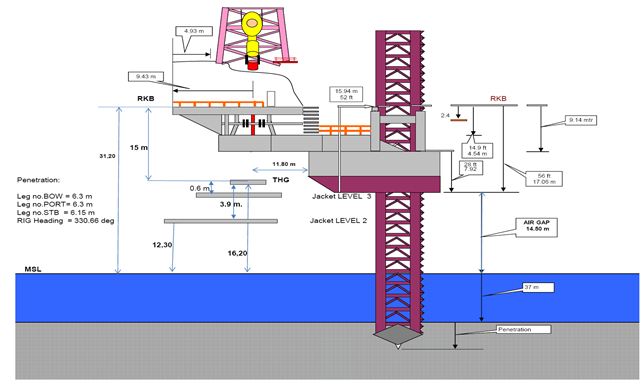
A jackup rig is required to drill well 317 in the Black Sea, Romania. The jackup had to be moved from PORT PL8 on the shore of the Black Sea to a location of PFS8 well 317 in order to be installed starting from the 3rd march 2020. The configuration and components of jackup are shown in Figure 4. Positioning survey will provide constant data showing the position of the unit at all times during the operation, with particular respect to protection of the integrity of sub-sea assets. This will also help to maintain recoverable records throughout the operation. Moreover, this will allow to advise the Tow Master and report to the Marine Representative throughout the operation. Data of location departing are illustrated in Table 1. On the other hand, data of location arriving are demonstrated in Table 2. For insurance purposes of towing vessels, the minimum requirement is a minimum of Tugs: GSP Antares 18000HP / 170 TBP. Also, for departure - 2 harbour tugs package are required. Assisting tugs should carry minimum one soft/hard eye pennant in order to connect to the stern. If practical the towing vessels and their equipment should be inspected by the attending Tow Master. Lead Tug to present Tow Master (who will consult with the OIM) intended Tow-Route / Passage Plan for approval. For more details about towing operations, Table 3 is provided.
| Designation | PORT PL8 |
|---|---|
| Coordinates | 440 05’ 48.82” N |
| Water depth | 7mtrs |
| Seabed data | Mud /SAND |
| Penetration | 4mtrs |
| Prevailing current | N/A |
| Prevailing wind | S- W / N-E |
| Air Gap | 2mtrs |
| Obstructions | - |
| Remarks | Legs should have a sufficient clearance from seabed before departure. |
Table 2: Location Departing.
| Designation | PFS 8 well 317 | |
|---|---|---|
| Unit co-ordinates WGS 84 | Lat:440 35’ 59.59” N Long:0290 21’ 31.58” E | |
| Water depth in meters | 37 m | |
| Soil data | Sand/Clay | |
| Expected Penetration | 6 mtrs-7 mtrs | |
| Prevailing current | NE/SE | |
| Prevailing wind | S-W / N-E | |
| Tidal range | N/A | |
| Time of High water at Location | N/A | |
| Rig Heading | 332(+/- 002) deg TRUE | |
| Obstruction | PFS 8 structure, pipes, cables underneath of the rig | |
| Remarks | ||
| Towing distance | 48 NM | |
| Towing route | - | |
| Estimated full towing speed | 4.0 Knots | |
| Average towing speed | 3 Knots | |
| Time break down | Estimate | PFS 8 |
| Jacking down, integrity check, move out of PORT FP8 | 4 | 4 |
| Estimated towing time | 16 | 20 |
| PFS 8– Positioning | 12 | 32 |
| Require window | 32HRS | |
Table 3: Location arriving.
Results and Discussions
In order to study the action of marin environment on jackup rig, it is necessary to review, firstly, the procedures of departure, transit, and emplacement on any emergency jacking location / stand by location as follows:
Departure Procedure
- Prior to departure a meeting will be held on board of the rig with all parties involved.
- Departure Draft max. 5 m.
- Survey gear will be installed configured, calibrated.
- Stability calculation to be in place.
- Towing Bridle to be in ∆ ended in single leg.
- Permission to be obtained from Port Authorities to depart.
- Final checks, according the ‘Rig’s Check List’.
- As soon as move crew arrived onboard, a muster and toolbox meeting with the full crew as a pre job meeting will be held with all personnel involved. In which meeting the jacking operation and procedures will be discussed as a risk assessment held for the planned move.
- As soon as the sea tugs arrive, Tow Master will inspect the vessels and brief the masters.
- Departure time to be scheduled. Pilot and Tow Master on board of the rig.
- As soon as a weather window appears, timing to be discussed, this includes the time to free the legs, which is anticipated to take several hours. Planned to be done on forehand. Operation will start well in advance before departure. Leading tugs will be connected.
- Rig will jack down into the water for a water tight integrity check.
- As soon as the water tight integrity is checked, hull will be lowered until floating draft, pulling legs until they indicate that they do not stick.
- Harbour tugs connected on pilot indication.
- Legs will be raised, rig will be pulled off the shipyard location.
- When unit is 500m out of break water point the convoy to be turned towards PFS 8 according with Towing Appendix.
Transit Procedure
- Tugs configuration to be changed, if required. Tow will set course to the new location.
- When convoy is in clear area, the Tow Master may hand over the command of the convoy to the lead tug. Length of tow line will be adjusted, if applicable.
- Navigational warnings should be transmitted at regular intervals throughout the passage by the leading tug to warn other vessels of the rig position and progress.
- Weather forecast will be studied upon receipt and decision to be made either to continue or to steam up to the standby location.
- Passage will be reviewed after each forecast either to continue to the Intermediate Position.
- All shipping lanes to be crossed at right angles in accordance with maritime rules (Vide ‘International Regulations for preventing Collisions at Sea – IMO904E).
Emplacement on any Emergency Jacking Location / Stand by Location
- When the rig is forced to jack up at any intermediate location: The tugs will be warned.
- The rig will be prepared to jack down; Survey gear made ready to do a final survey;
- Toolbox meeting with crew to discuss operation.
- Rig will approach the particular location, at 2 NM distance tugs will shorten wires to approx. 300m.
- Whenever the Tow Master feels the need, he might decide to re-position any vessel.
- Tow Master will guide the rig against the wind and current and will steam slowly towards the location, this while the legs are lowered down to 2m of the seabed. The water depth will be checked throughout the operation.
- Minimum speed will be maintained for this last part of the approach. In position, approximate 100 to 500 m from the original location, rig will be kept stationary.
- When the seabed seems to be clear of debris, legs will be lowered for the last 2m.
- When the rig is pinned, hull will be raised out of the water.
- Normal pre-drive procedures will be followed.
- Authorities will be notified. Tugs could be disconnected / released.
- When the next proper weather window appears, the unit will leave the emergency location.
- Rig will jack down to 3m air gap, tugs will be connected.
- Unit will be lowered in the water (1.5m) for a water tight integrity check.
15. When all check O.K., tugs will take positions and hull will be lowered to draft. 16. Legs will be pulled free from the seabed and raised to the required height. 17. Unit will resume passage to the final location.
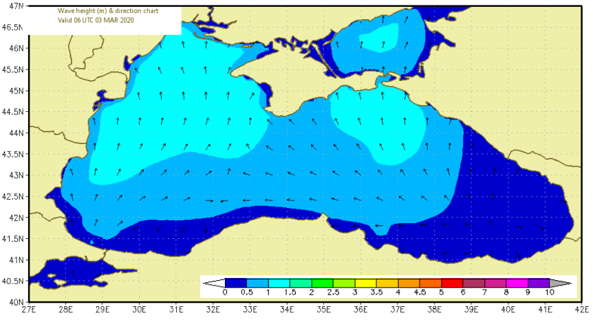
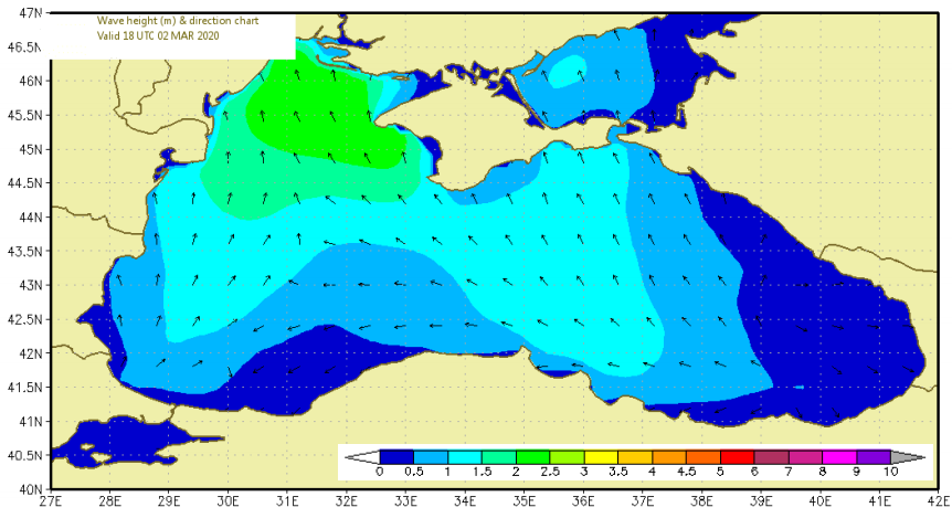
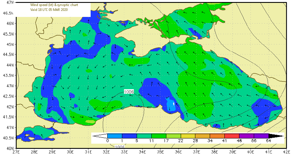
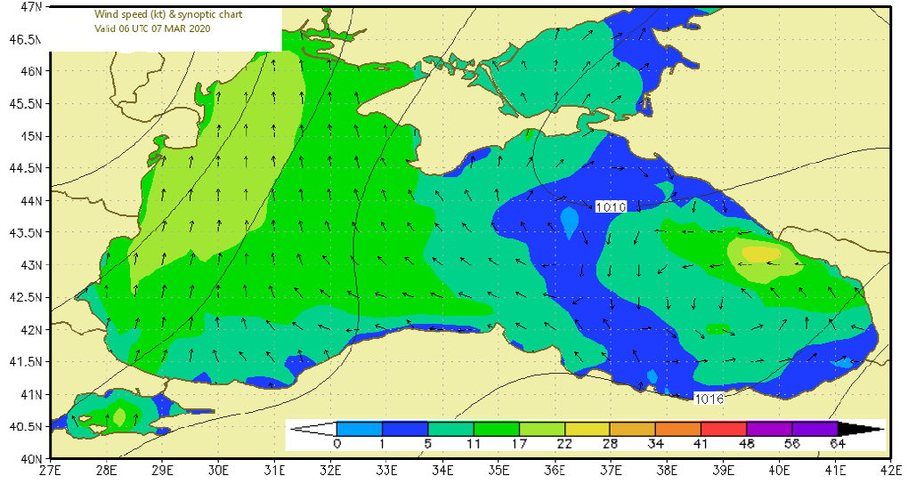
Secondly, weather forecasting is the first step to study the action of marine environment on the jackup rig. The conditions of weather forecasting are predicted and computed starting from the 2nd March and for the next four days when the jackup is installed. It was found that:
On 03 March 2020
- Weather Forecast for Mid-point at 44.5N 29.5E Subject:
- Validity: Forecast valid 120 hours from 0600 (UTC+
- on 03 Mar 2020
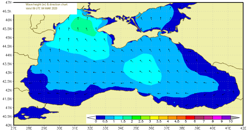
On 04 March 2020
- Subject: Weather Forecast for Mid-point at 44.5N 29.5E
- Validity: Forecast valid 120 hours from 0600 (UTC+
- on 04 Mar 2020
On 05 March 2020
- Subject: Weather Forecast for Mid-point at 44.5N 29.5E
- Validity: Forecast valid 120 hours from 0600 (UTC+
- on 05 Mar 2020
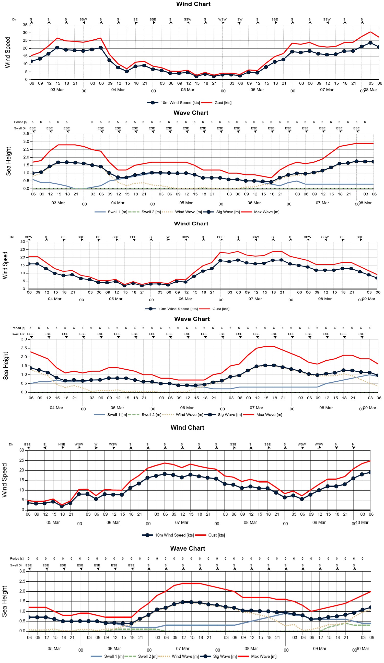
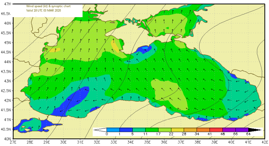
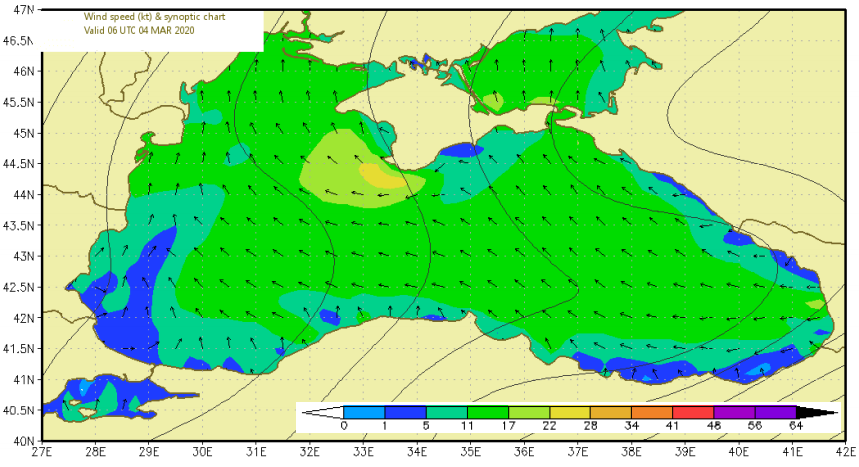
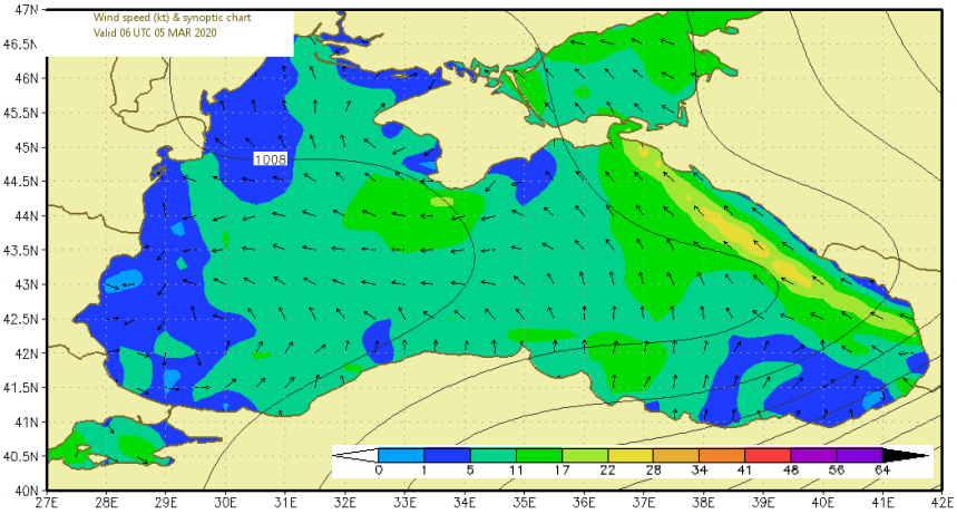
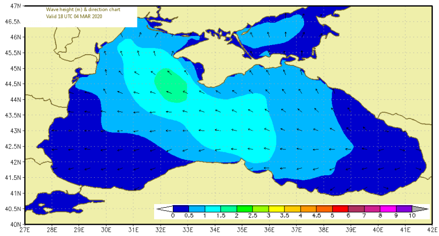
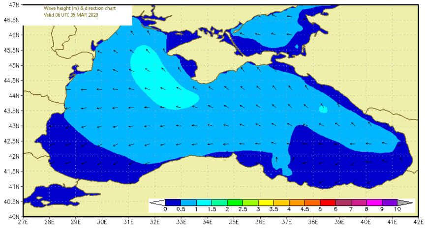
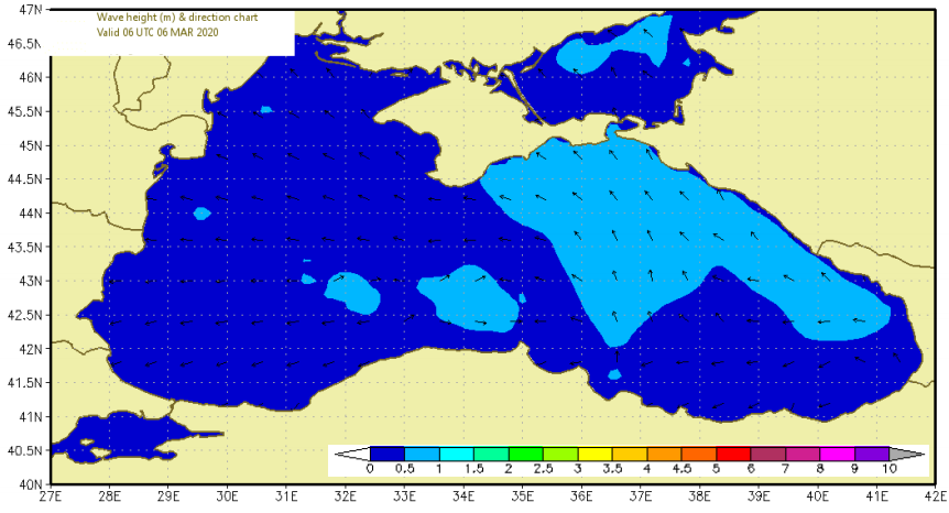
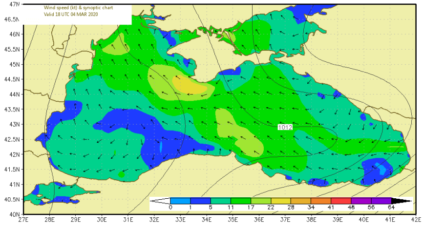
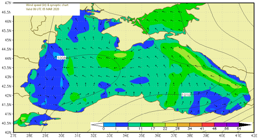
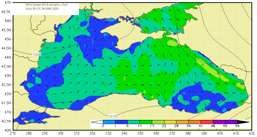
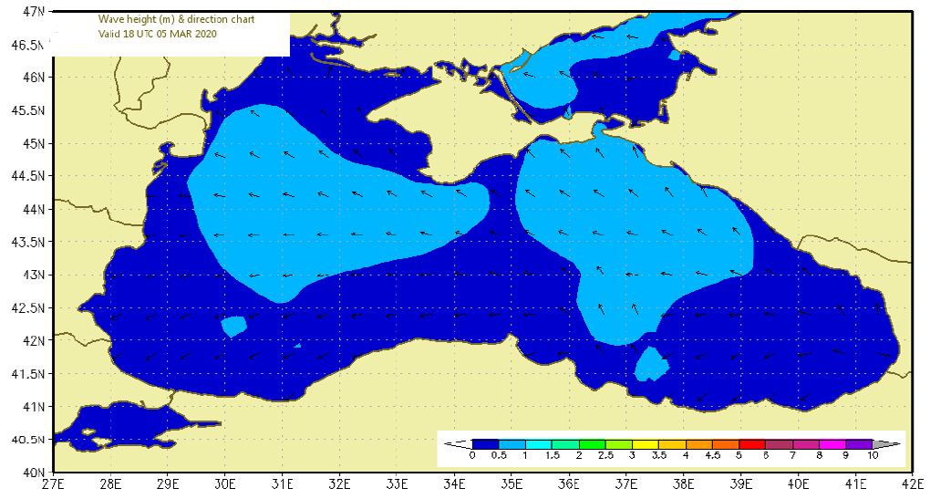
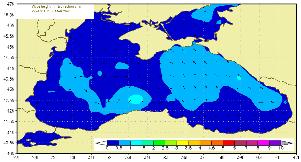
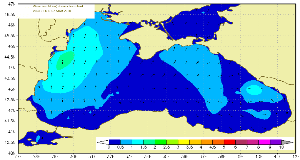
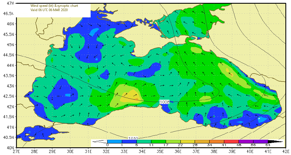
Figures 5-11 shows the action of marine environment on jackup rig during its installation. On the 3rd March, it was found that fairly high for trend, but moderate for peak wind/wave detail is appeared due to a ridge extending nearby. Falling low overall by late period. Stronger shower gusts. However, fairly high for trend, but moderate for peak wind/wave detail is appeared from the next day onwards as a trough deepens across the area. Low overall by late period. Stronger shower gusts. On 5 March, fairly high for trend, but moderate for peak wind/wave detail is occurred as a complex low fills close to your area. Moderate overall by mid period and low overall by late period. Stronger shower gusts.
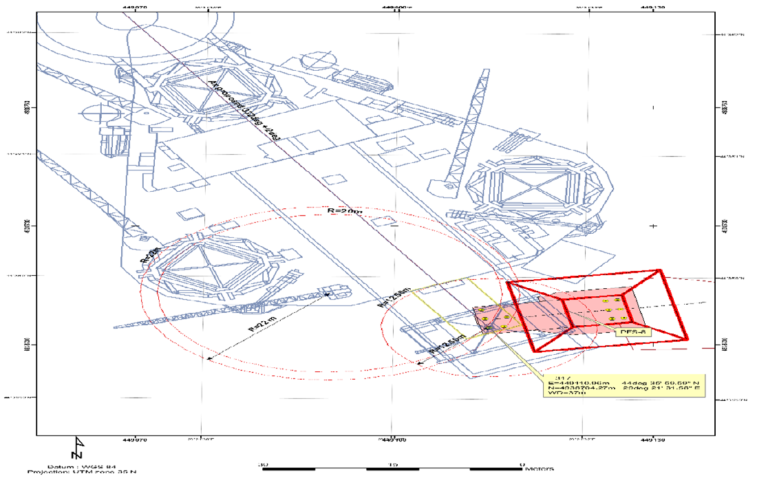
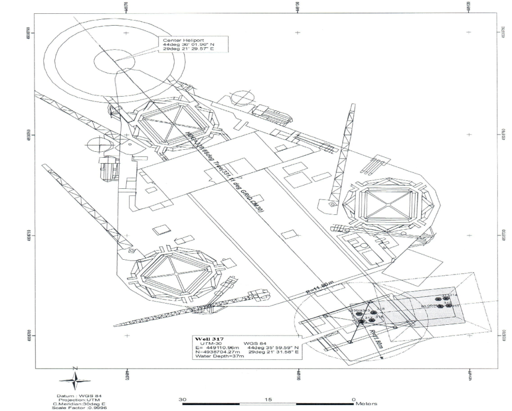
Based on the data provided from the positioning survey and Tables 1 & 2, the jackup rig is positioned in its location safely with the following results (Figures 12 & 13):
Intended offset/well location: 317-FPS8
Surface Co-ordinates Datum WGS 84 Latitude 44o 35’ 59.59” (N) Longitude 029o 21’ 31.58” (E) Projection Transverse Mercator CM=30o E TM(CM=27°) Easting=449110.96 m Easting=687197.50 m Northing=4938704.27 m Northing=4941210.70 m Intended rig heading is at 332° (+/-2°) True
Final rig position for well 317 surface
UTM’s WGS 84 Easting=449110.96 m Latitude=44° 35’ 59.59” (N) Northing=4938704.27 m Longitude=029° 21’ 31.58” (E) 1. Rig heading: 330.66° True (331.11° Grid TM30):
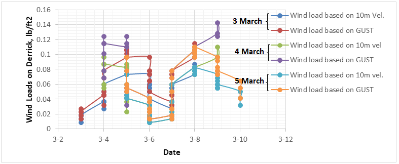
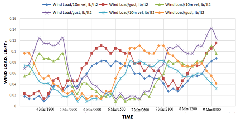
Convergence=-0.450° world standard 2. Water depth is 37 m 3. Centre Heliport of the jackup Latitude=44° 36’ 01.96” (N) Longitude=029° 21’ 29.57” (E) Wind loads are computed based on the 10m sustained wind and gust velocities for the predicted period starting from the 3rd March to the 5th March 2020 and for the next 5 days. The results are shown in Figures 14 & 15 which are plotted based on date and time. Clearly, it`s appeared that there a discrepancy in the predicted values for the 1st third of March. On 3 March, the predicted wind loads affected on derrick are low compared with 4 and 5 March at the first period. However, they increase and record higher values more than ones predicted for the other 2 days. At the end of period, they are relatively high but still less than those of the other 2 days.
Conclusions and Recommendations
A study of the impact of marine environment on a jackup rig was implemented in paper. The developed results are effectively predicting the safe conditions and optimizing the positioning survey of the rig. Also, the following conclusions are extracted based on the predicted conditions and results:
- Towing process is highly affected by the weather conditions
- Defining the procedures of departure, transit, and emplacement on any emergency jacking location / stand by location enhances the safety of operations
- Weather forecast is a main factor in determining the action of wind, and waves on jackup
- Changing wind directions leads to a change in its velocity, height, and impact on jackup rig. And the same for waves.
- Wind loads on derrick is significantly changed by alterations of weather conditions
Nomenclatures
| A | Projected area of a member taken as the projection on a plane normal to the direction of the considered force |
|---|---|
| Al | Parameter of P(√E) |
| a | Elementary wave amplitude |
| B | (σ/A1)2 |
| b | Parameter of P(a) |
| C | Shape coefficient (3-dimensional flow) |
| C∞ | Shape coefficient (2-dimensional flow) |
| CD | Drag coefficient |
| CH | Height coefficient |
| CM | 1 + Cm (inertia coefficient) |
| l | Wave train number |
| M | Parameter of P(√E) |
| MT | Total overturning moment on a large volume structure |
| P(σ) | The long term Weibull distribution of the response amplitude σ |
| Ps(σ ) | The short term Rayleigh distribution of the response amplitude σ |
| P(√E) | The long term Weibull distribution of √E |
| P(√E) | dP(√E)/ dP √E |
| P(H) | Long term Weibull distribution of individual wave heights |
| P(Hv) | Long term Weibull distribution of visually observed wave heights |
| RE | VD/γ Reynold’snumber |
| SR2 | Area beneath the response spectrum curve |
| SW2 | Area beneath the wave spectrum curve |
| SR(ω)2 | Response spectrum |
| SW(ω)2 | Two-dimensional wave spectrum |
| SW(ω,α)2 | Three-dimensional wave spectrum |
| T | Zero-uncrossing period |
| T | Average apparent zero-upcrossing period |
| Tm | Peak period of the wave spectrum |
| t | Time interval |
| T R | Average apparent zero-upcrossing period of the response amplitude σ |
| V | Water particle velocity due to wave and current |
| V | Water particle acceleration due to wave |
| Vcy | Total current velocity y meters above sea bottom |
| VT | Tide-induced current velocity at sea surface |
| VW | Wind-induced current velocity at sea surface |
| Vz | Sustained wind velocity z meters above sea surface |
| (Vz)G | Gust wind velocity z meters above sea surface |
| V10 | Sustained wind velocity at 10 meters above sea surface |
| Cm | Added mass coefficient |
|---|---|
| D | Diameter |
| d | Cross sectional dimension normal to the direction of the considered force |
| E | Parameter of the short term Rayleigh distribution |
| E(f) | Wave spectrum as a function of frequency f (hz) |
| FH | Total horizontal force on a large volume structure |
| FW | Wind force acting perpendicular to an area A |
| FY | Wind force acting in direction of the wind |
| F(α) | Directionality function |
| f | Frequency (hz) |
| fm | Peak frequency of the wave spectrum (hz ) |
| g | Acceleration due to gravity |
| H | Individual crest-to-trough wave height |
| H1 | Still water depth |
| Hc, Ho, G | Parameter of P{Hv)’ |
| Hv | Visually observed wave height |
| H1/3 | Significant wave height |
| Hmax | Most probable largest wave height |
| i | Wave frequency number |
| K | Parameter of P(α) |
| k | Wave number ( 2π/r ) |
| L | Length of member |
| ΔL | Length of element or portion of structure considered |
| V10 | Sustained wind velocity at 10 meters above sea surface acting normal to an area, A |
|---|---|
| Y | Transfer function |
| y | Distance above sea bottom |
| z | Distance above sea surface |
| α | Angle between main direction of propagation of short crested wave system and the elementary long crested wave systems |
| α1 | Angle between velocity vector and axis (or surface) of member |
| β | Heading angle |
| β1 | Angle between acceleration vector and axis (or surface) of member |
| λ | Wave length |
| ω | Circular wave frequency |
| σ | Elementary response amplitude |
| ζ | Phase angle |
| ξ | Density of fluid |
| γ1 | Kinematic viscosity |
| γ | Peakedness parameter |
| Draft | Depth of submerged hull |
| LCB | Longitudinal center of buoyancy |
| VCB | Vertical center of buoyancy |
| LCF | Longitudinal center of floatation |
| Displacement | Weight |
| KML | Longitudinal metacentric height above keel |
| K | Keel |
| KG | Vertical distance from keel to center of buoyancy |
| M | Metacenter |
| KMT | Transverse metacentric height above keel |
| MH1” | Moment to heel one inch |
| MT1” | Moment to trim one inch |
| TP1” | Tons per inch immersion |
| GZ | Heel lever arm |
| G | Location of center of gravity |
| Righting Moment | Displacement multiplied by GZ |
| Heeling Moment | Overturning moment produced by wind |
| Down flooding Angle | Angle of heel at which water will enter the hull through an opening |
| Second Intercept | Second crossing of righting moment and heeling moment curves |
| k | Constant, as defined by regulatory agency |
References
-
Laik (2018) Offshore Petroleum Drilling and Production. CRC Press, Taylor & Francis Group, LLC, pp: 1-649.
-
Austin EH (1983) Drilling Engineering Handbook. 1st(Edn.), Springer Netherlands, Boston, USA, pp: 301.
-
ETA Offshore Seminars (1976) The Technology of Offshore Drilling, Completion and Production. PennWell Publishing Company, USA.
-
Rules for the Design, Construction and Inspection of Fixed Offshore Structures, Norske Veritas (Oslo).
-
Rules for the Construction and Classification of Mobile Offshore Units, Det norske Veritas (Oslo).
-
Davenport AG (1960) Wind Loads on Structures. National Research Council, Division of Building Research, Technical, pp: 88.
-
Pierson WJ, Moskowitz L (1964) A Proposed Spectra Form for Fully Developed Wind Seas Based on the Similarity Theory of S. A. Kitaigorodskii. Journal of Geophys Res 69(24): 5181-5190.
-
Wind Statistics for the North Seaand the Norwegian Ocp. an. Det norske Veritas Report, pp: 74-53.
-
Hossain ME, Al-Majed AA (2015) Fundamentals of Sustainable Drilling Engineering. John Wiley & Sons, pp: 786.
-
Liu G, Li H (2017) Offshore Platform Integration and Floatover Technology. 1st (Edn.), Springer Tracts in Civil Engineering, Springer Singapore, pp: 280.
-
Halafawi M, Avram L (2018) Well Integrity, Risk Assessment and Cost Analysis for Petroleum Fields and Production Wells with CO2. International Journal of Innovations in Engineering and Technology 10(4): 39- 52.
-
Halafawi M, Marius S, Avram L (2019) Prediction Modelling for Platforms’ Network Vessels Performance. Petroleum and Coal Journal 61(5): 983-997.
- Nigeria’s Vulnerability in the Face of Global Energy Policy
- A Simulation Study of Investigation of Optimum Oil Production Performance by Applying Various Gas Injection Methods in Oil Reservoir
- Characterization of Permo-Triassic Reservoirs through Thermal Maturity Assessment of Westphalian Source Rocks in the Cheshire Basin
- Influence of Microwax on the Rheological and Thermal Behaviour of a Wax Crude Oil
- Real-Time Monitoring and Performance Optimization of Steam Injection in Heavy Oil Reservoirs Using Fiber Optic Sensing and Integrated Predictive Simulation Models
- Rapid On-Site Determination of the Total Petroleum Hydrocarbon Content of Soils by Handheld Fourier Transform Near-Infrared Spectroscopy: Development of a Global, Site- and Scanner- Independent Calibration Model