Efficiency of the Simulated Annealing Algorithm in Solving the Traveling Salesman Problem

Introduction

Simulated annealing is an optimization technique which has been used to obtain the optimal solution in many problems [1] including the traveling salesman problem [2, 3]. In this study we focus on the efficiency of this technique when compared with the brute force technique.

In the simulated annealing technique [1], the system is initially at a high “temperature” and an initial random configuration is generated. Slight changes in configuration are made and the new configurations are either accepted Perspective or rejected by following the Metropolis algorithm [4]. After generating a certain number of configurations, the “temperature” of the system is lowered and the process is repeated. According to the Metropolis algorithm, most configurations are accepted when the system is at a high temperature, while the acceptance ratio goes down as the temperature is reduced. When the temperature has been reduced to a very low value, the system would have settled down close to the optimal configuration. The total number of configurations which are generated will obviously have a bearing on the error associated with the final result of the algorithm. If a sufficiently large number of configurations are generated, the final configuration is expected to be close to the optimal solution, while the error is expected to increase as we reduce the total number of configurations. The main motivation of this study was to study the error as a function of the number of configurations and also to see whether reasonable results can be obtained by using a number of configurations which is much smaller than the n! configurations (n being the total number of cities) which a brute force algorithm would require.

Simulated annealing has been studied extensively and applied to a variety of systems since the original paper by Kirkpatrick etc al. [1] in 1983. A recent review of simulated annealing as well as other nature-inspired metaheuristic algorithms can be found in the review by Xin-She Yang [5]. Two commonly used annealing schedules are linear and geometric [5]. Recently a list- based simulated annealing algorithm has been proposed which uses a list of temperatures for the cooling schedule [6]. Attempts have also been made to use the greedy search algorithm with simulated annealing [7].

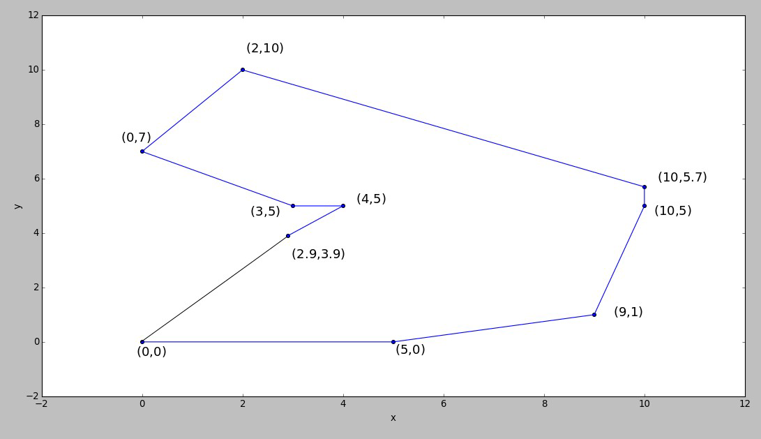
For testing the efficiency of the simulated annealing method in solving the traveling salesman problem, we considered a collection of 10 “cities”. The coordinates of these cities were chosen randomly. The x and y coordinates of these 10 cities were [[0, 0], [10, 5.7], [2, 10], [0, 7], [5, 0], [3, 5], [9, 1], [10, 5], [2.9, 3.9], [4, 5]]. We wrote a program which would generate all the 9! configurations possible for these 10 cities. We generated only 9! configurations as the salesman is supposed to start from a particular city and return to the same city. The brute force algorithm gave the length of the shortest path which traversed all the 10 cities as 37.655. Figure 1 shows the optimal solution given by the brute force algorithm.

Pseudo-code for Simulated Annealing Algorithm

1. T=Tmax
2. Max accepted=10*n
3. While (T>

$$ \begin{array}{l} \mathrm {I f} \mathrm {E} \left(\mathrm {C} _ {1}\right) < \mathrm {E} \left(\mathrm {C} _ {0}\right) \\ \mathrm {C} _ {\mathrm {g}} = \mathrm {C} _ {1} \\ a c c e p t e d + + \\ \end{array} $$

else if(C1>C0) and If (e-(E(C1)-E(C0))/KT>random(0,1))

Cg=C1 accepted++

If accepted>Maxaccepted break

T=T-dT

If accepted==0 break

4. Return Cg.

Results obtained using Simulated Annealing and Analysis of Results

Click to enlarge

In our simulated annealing method, the Boltzmann factor was taken to be exp(-E/T), i.e, the Boltzmann constant was taken to be equal to unity. The “energy” E is nothing but the total path length for a certain path which passes once through all the cities.

The initial temperature should be chosen to be much higher than the optimum value of E. Since the optimal solution was already known to be 37.655, we chose the initial temperature to be 200.

We repeatedly implemented the simulated annealing algorithm for varying number of iterations and determined the percentage error in the final solution given by the algorithm (when compared with the brute force solution).

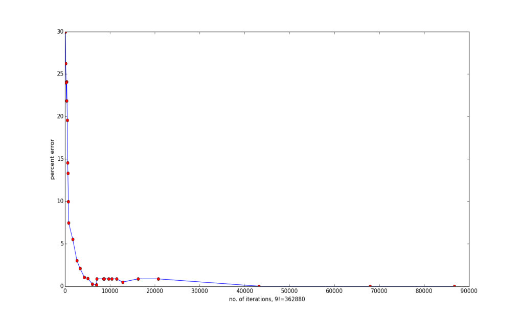
Figure 2 shows the plot of error in the final solution obtained by the simulated annealing method as a function of the total number of iterations performed by the algorithm to obtain the solution.

Click to enlarge

0 A B C D

We believe that since the coordinates of the cities were chosen randomly, the results obtained by us are valid in general. Further, we can understand the dramatic decrease in the error (when the number of iterations is increased) by a simple qualitative argument.

We use Figure 4 to present our qualitative argument. Since the initial configuration is chosen randomly it has a 50% chance of being in the region BC. In the Figure 3, all possible values of E (total path length) are marked by points on a number line Figure 3: 4 points path length.

Here A represents the length of the shortest path and D represents the length of the longest path for the given configuration. Assuming that the points which represent various possible configurations are spread uniformly over the range AD, we can say that a random configuration is most likely to be in the range BC, where AB and CD are ¼ th of the range AD. As we generate many different configurations and also lower the temperature, the system would “move” from its initial configuration towards the point A. Of course this would not be a unidirectional motion as the simulated annealing algorithm has some probability for accepting a configuration which has a higher value of E. If our algorithm generates a sufficient number of configurations, then in all those cases, the final configuration is very close to A and the error is negligible. This is why the error is negligible when the total number of iterations is in the range 90,000 to 10000. However, when the number of iterations drops below a certain value then the final configuration is far from the point A and the error rises dramatically when we reduce the number of iterations. Assuming a uniform distribution of points (path lengths) on the number line, we would expect a linear relation between the error and number of iterations. It can be seen that the data in Figure 2 can be fit to two separate straight lines one for the range 0-5000 iterations and the other (a straight line of almost zero slope) for the range 5000-90000.

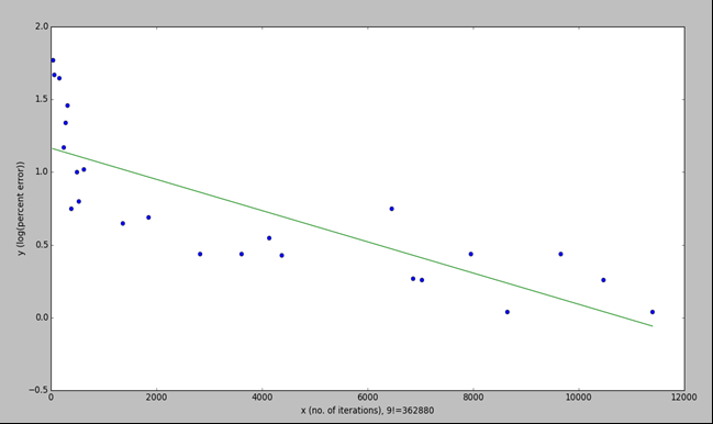
It can be seen from a semi-log graph (see Figure 4 below) of the data in Figure 2 that the error does not decrease exponentially with an increase in number of iterations.

Click to enlarge

References

-
Kirkpatrick S, Gelatt CD, Vecchi MP (1983) Optimization by Simulated Annealing. Science 220(4598): 671-680.
Černý V (1985) A thermodynamical approach to the travelling salesman problem: An efficient simulation algorithm. Journal of Optimization theory and applications 45(1): 41-51.
Geng X, Chen Z, Yang W, Shi D, Zhao K (2011) Solving the travelling salesman problem based on adaptive simulated annealing algorithm with greedy search. Applied Soft computing 11(4): 3680-3689.
Metropolis N, Rosenbluth AW, Rosenbluth MN, Teller AH, Teller E (l1953) Equations of state calculations by fast computing machines. Journal of Chemical Physics 21**:** 1087-1092.
Xin-She Y (2010) Nature-inspired metaheuristic algorithms. 2nd (Edn.), Luniver press, UK, pp: 1-75.
Zhan SH, Lin J, Zhang ZJ, Zhong YW (2016) List-based simulated annealing algorithm for traveling salesman problem. Computational Intelligence and Neuroscience, pp: 12.
Wu X, Gao D (2017) A Study on Greedy Search to Improve Simulated Annealing for Large-Scale Traveling Salesman Problem. International Conference in Swarm Intelligence, pp: 250-257.
- Sense, Gravity, Parity & Chirality in Mathematical Physics
- Quantum Lattice Simulations PHYSICS: Microcircuit Particle Formation and Observable Macroscopic Irreversible Time - A Discrete Lagrangian with Cellular Automata Framework
- Quantum Biology from Biomacromolecule to Cell, and Central Dogma Described by Quantum Theory
- Focus, Agility, Speed and Technology (FAST) for Sustainability and Growth
- Square Root Metric Geometry and Pati-Salam Model in Curved Space-Time
- A Simple System Demonstrating the Mpemba Effect in Classical Mechanics