Reformulating the Basics of Conventional Newtonian Physics, Quantum Physics and the Einstein Theories of Relativities Based on the newly discovered Topological Theory of Quantum Gravity (TTQG)
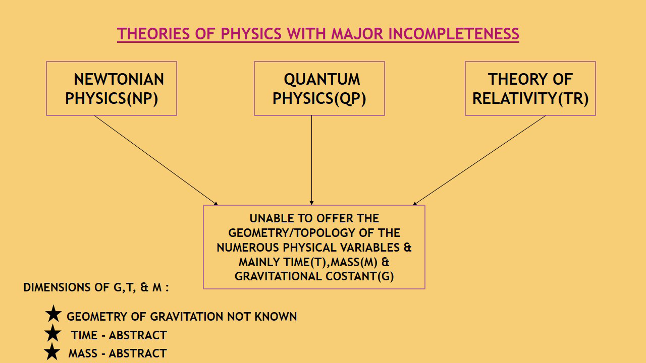
The Newtonian physics, quantum physics and the theories of relativity suffer from a major Incompleteness on the ground of being unable to offer the topologies and the dimensionalities of the numerous physical variables. Out of the three very familiar dimensions of physical variables in conventional physics length (L), mass (M) and time (T), the two variables, namely mass and time are fully arbitrary and abstract. In Newtonian physics L, M and T are fully independent variables since no mathematical equation linking the said three variables have been proposed. It is an established fact and a matter of everyday experience that L, M and T are very much linked to each other and otherwise which, the universe could have taken either the infinite number of shapes of desire arising out of endless permutations and combinations of L, M and T or could have merged to fully length (LM°T°) or fully mass (L°MT°) or fully time (L°M° T). Max Planck tied up the five numbers of basic physical variables, length, time, mass, electric charge and temperature to the same source by linking all of them to the Newton’s Gravitational constant (G) and Planck constant (h). However, this attempt was also incomplete since the topologies of G and h, could not be put forward. Later on, the quantum physics even, could not erase the stamp of ‘abstractness’ as put on the physical variables like mass, time, temperature, gravitation, photon waves and many others. Neither the Newtonian physics nor the quantum physics can depict the dimensionalities of entropy, force, energy, acceleration, black hole, plasma state, etc. and as well cannot also tell us how a ‘photon’ looks alike or what the ‘gravitons’ are in reality. The recently discovered topological theory of quantum gravity (TTQG) revealed the following: 1. The phenomenon of gravitation is being linked to the intermolecular attractive forces. 2. Have defined all the above said physical variables as ‘gravitons’ in regard to entropy. 3. Presented the topologies and dimensionalities of the physical variables. 4. Introduced the inverse dimensionality concept in physics. 5. Proposed the mathematical equation relating L, M and T 6. Reformulated the basics of Newtonian physics, quantum physics and the special and general theories of relativity. 7. All the cosmic phenomena of the universe have been represented by a singularity graviton originated universal graviton cycle.
Dimensionalities and Topologies of the Physical Variables of the Universe
The dimensionalities and the topologies of the physical variables of the universe as evaluated in TTQG is shown below in Figure 2:
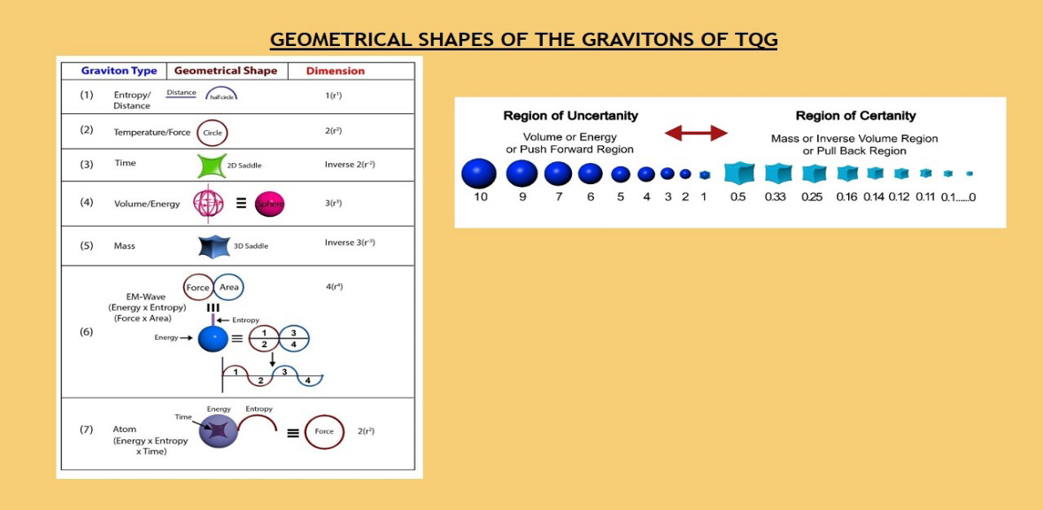
This is well known fact that neither the Newtonian Physics (NP) nor the Quantum Physics ( QP) could depict the dimensionalities of entropy, force, time, temperature, energy, electromagnetic- wave, acceleration, black hole, plasma stat, etc.
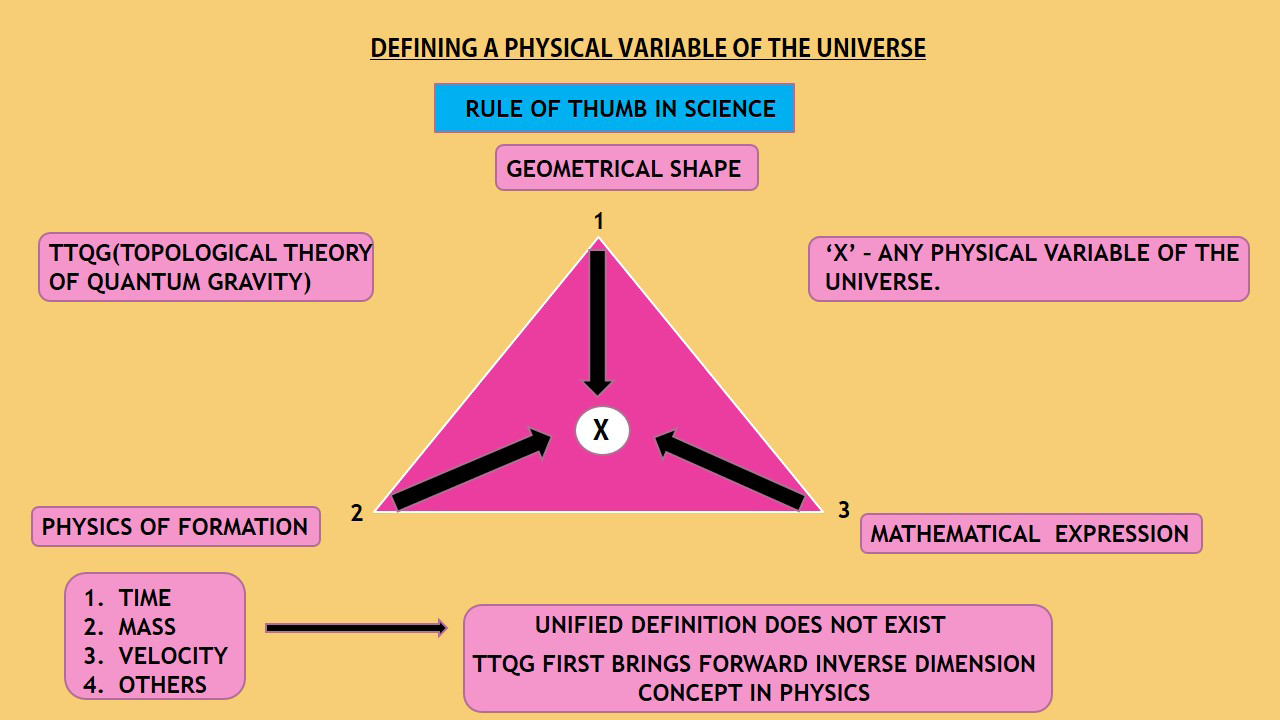
The none of the streams of physics NP, QP or the GTR can tell us what the ‘gravitons’ are or how does a ‘photon’ look alike. One needs to follow first in this context, one of the principal philosophy of TTQG for defining a physical variable and which is being shown in Figure 3 below:
TTQG defined the cosmological variables in terms of ‘ENTROPY’, the most significant thermodynamic parameters and also has depicted the geometrical shapes of the physical variables. TTQG POSTULATES [98, 99, 100, 101, 102]: 1) Molecular attractive forces are the origin of gravitation.
2) Molecular attractive forces are linked to intermolecular distance (r). 3) Entropy is an integral multiple of r. 4) Time has inverse dimensions of a circle, which is a 2D saddle and time is an inverse force holding the universe. 5) Energy and volume are indistinguishable by their dimensions. 6) Gravitation is the result of overlapping of two inverse acceleration field and its predicted extremely cohesive or attractive geometry firmly establishes this as singularity gravitons.
Here it will be shown how the concepts of ‘time’, ‘mass’ and ‘gravitation’ are derived in TTQG. To understand this one needs to understand the following two phenomena:
- ‘Entropy’ is unidimensional physical variable
- ‘Pressure’ is dimensionless physical variable The classical physics cannot offer the absolute dimension of a physical variable except solely the length or the length based physical variables like area or volume. The dimensions of most of the physical variables of the Newtonian or classical physics ( with which we are accustomed to) are very relative ones since the dimensions of time, mass, gravitation, velocity are not defined. In TTQG the absolute dimensions of the physical variables have been evaluated in terms of entropy (distance), force (area) and energy (volume). ‘Space’ is volume and ‘space’ is the infinite store of energy. The volume is defined as the amount of space and so volume and energy are dimensionally indistinguishable or have the same dimension.
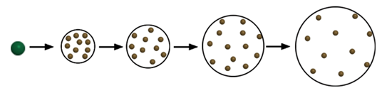
As far as the concept of modern cosmology [4, 5, 6, 7, 8, 9, 10, 11, 12, 13, 14, 15, 16, 17, 18, 19, 20, 21, 22, 23, 24, 25, 26, 27, 28, 29, 30, 31, 32, 33, 34, 35, 36, 37, 38, 39, 40, 41, 42, 43, 44, 45, 46, 47, 48, 49, 50, 51, 52, 53, 54, 55, 56, 57, 58, 59, 60, 61, 62, 63, 64, 65, 66, 67, 68, 69, 70, 71, 72, 73, 74, 75, 76, 77, 78, 79, 80, 81, 82, 83, 84, 85, 86, 87, 88, 89, 90, 91, 92, 93, 94, 95, 96, 97] is concerned on a large scale structure, the universe is isotropic and homogeneous in regard to energy. This means that the matters grow equally in 3 mutually perpendicular directions (x, y & z) and the volume which we observe is the overlapping of the equal volumes (V) of the 3 directions. So energy (E) is defined in TTQG as the summation of the 3 numbers of such equal volumes such that E=3V. TTQG has established this diagrammatically in Figure ( 4a,4b &4c) below:
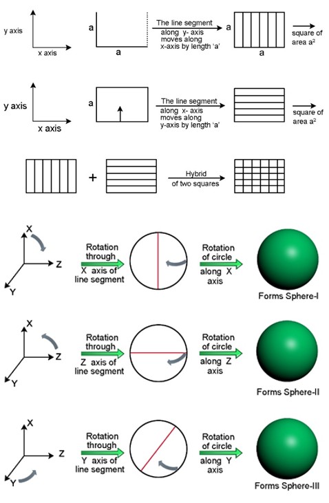
Figure 4a: Hybrid concept of formation of a square.
Figure 4b: Formation of a sphere by rotation of line segments & circles along 3 principal directions X, Y & Z.
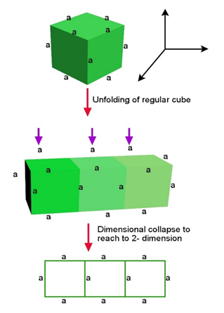
Figure 4c: Dimensional collapse of a cube after unfolding.
From Figure 4 it becomes very much evident that a spherical space what we observe is inherently an overlapping space of the volumes of the 3 directions or one can say that a sphere contains 3 spheres (as shown in Figure 4b, sphere I, sphere II and sphere III). If the volume of each sphere is being considered V, the energy of the sphere will be 3V under the condition of equilibrium with the surroundings.
Now, the parameter pressure (P) needs to be understood very well. In any matter of the universe among the molecules push forward forces (repulsive forces) and pull back forces (intermolecular attractive forces) are operating. Pressure of a substance is the hybrid of the “PUSH FORWARD FORCE” and the “PULL BACK FORCE”. This can also be called as the hybrid of kinetic (push forward) force and the potential (pull back) force. Such that the Pressure (P) can be written as P = [Push forward force (PFF)] x [Pull back force(PBF)] (1) Boyle’s law is very well known and ancient law of physics, which states, pressure (P) is inversely proportional to volume (V) when temperature (T) is constant.
( ) ( ) 1 P V α (2)
Or PV = K = Boyle’s constant The unit or dimension of pressure in conventional physics is ‘energy per unit volume’. So the Boyle’s law can be stated in the following way.
(energy /volume) α (1/ volume) (3)
The above equation is not acceptable as far as the theory of mathematical variation is considered. If for example, X and Y are two variables, it does not carry any sense to express the proportionality relation between them in the following manner in equation (4) (since both the RHS and LHS contain the same variable Y) ( ) ( ) X/Y 1/Y α (4) In this context it is to mention here very much that the unit of pressure as we know in the form, energy per unit volume, is not acceptable. In fact ‘pressure’ is a dimensionless parameter as explained below. The volume of a system (TV) is the sum of ‘Free volume’ (FV) and ‘Hard core volumes (HV) of all the molecules of the system as expressed in the form TV = (FV + HV) (5) Now in the case of a gas, as is illustrated in Boyle’s law, at a constant temperature, when pressure is increased the volume decreases and when the pressure is lowered, the volume increases and these are the fact of every day or common experience of every one. So the pressure of a system is in fact related to the ratio of the ‘HV’ to the ‘TV’ of a system. However, the Boyle’s constant, in fact represents the ‘hard core volume of all the molecules of a system’ and which is constant for a finite fixed quantity of as for example, a gas. So pressure P is in fact, a ratio of ‘Hard core volume’ to the ‘Total volume’ P = (HV/TV) (6) Since the pressure ‘P’ is a ratio of two volumes as shown in equation (6) above, it is a dimensionless parameter. ‘TV’ is related to the ‘FV’ as shown in equation (5). Pressure is bearing a inverse relationship to the free volume ‘FV’. When the ‘FV’ is higher, pressure is lower and when the ‘FV’ is lower, pressure is higher at a constant temperature. When the ‘FV’ is lower, the ‘push forward force, PFF’ is lower and when the ‘FV’ is higher the ‘pull back force, PBF’ is lower. So pressure P is a hybrid of ‘PFF’ and ‘PBF’ as shown in equation (1) above.
We often in science deal with “Randomness” and “Order” parameter of the matter/substances of the universe.
The actual definition of randomness is the homogenization of the push forward forces (directional force) generated among the molecules over the entire volume (V), by the multi-directional movement of the molecules.
Orderliness is the result of localization (inversion) of any directional force or pull back force, generated in a system owing to the presence of intermolecular attractive forces. So the energy of a system is a hybrid of PUSH FORWARD FORCE PULL BACK FORCE VOLUME And this needs to be considered for the entire 3 principal axis x, y and z respectively.
So energy over x- direction
= (PFF x PBF) x V
= PV
So the energy over all the 3 directions will be the
sum of PV for the 3 directions such that
$$ \mathrm {E} = \sum \mathrm {P V} $$ = 3PV Since pressure is dimensionless, energy and volume have the same dimensionalities, the product (PFF x PBF) has to be dimensionless and which is possible only when the pullback force is of inverse dimension of the push forward force. So as far as the relative units of NP are considered if the push forward force is expressed in dynes, the unit of pull back force would be (1/dynes).
In case of a system in equilibrium with the surroundings, the energy, (when P = 1) E = 3V or the energy density of space is constant in the form (E/V) = 3.00 When a substance is under equilibrium with the surroundings, this pressure, P is equal to unity. So P (equilibrium with the surroundings) = PFF x PBF = 1.00 (7) Now under non-equilibrium condition P = PFF x PBF can be either greater than 1 or less than 1.
If P < 1, then the substance, if being left on its own, starts contracting until or unless P becomes 1 and equilibrium is again attained.
If P >1, the substance starts expanding until and unless P becomes 1 and equilibrium is re-established. This is being illustrated in Table 1 below:
- Magnitude of Push Forward Force ( PFF)
- Magnitude of Pull Back Force (PBF)
- Magnitude of Pressure (P)= ( PFF x
- PBF)
- 10
- 10
- 1
- 20
- 10
- 2
- 10
- 20
- 0.5
Table 1: The variation of pressure with the magnitude of PFF and PBF.
Once establishing that pressure is a dimensionless parameter of the universe, we will evaluate the dimensionality of the most significant thermodynamic parameter ‘entropy’. Also to note that in TTQG all the physical variables of the universe has been expressed in terms of the average intermolecular distances.
The following figure (Figure 5) [98] is to note, which is representing in 2-dimension the expansion of a matter (for example upon heating) under constant pressure in equilibrium with the surroundings.
From the above figure it is very much clear that the average intermolecular distance increases as the volume increases or vice versa. Now if the circle’s average radius is considered to be r Then r = (n′-1)r′ ≈ n′r′ (for very large value of n′) When n′ is an integer 1, 2, 3, 4, 5, 6 and it represents the average number of molecules along any radius of the circle starting from the center of the circle, r′ being the average intermolecular distance. If this concept is being extended to 3-dimension, then one has to consider a sphere instead of a circle as shown in Figure 5.In that case, the higher the surface area of the sphere higher would be the randomness. Higher is the surface tension, lower would be the randomness. Higher be the ratio of surface area to surface tension, higher is the randomness and lower is the ratio of the said two parameters, lower is the degree of randomness. This ratio (surface area/ surface tension) is the actual index of randomness and we call it to be the absolute definition for “ENTROPY”.
Force = (Pressure) x (Area) = 2 1 4 x r π (8)
$$ \frac {F o r c e}{d i s t a n c e} = \frac {4 \pi r ^ {2}}{3 r} = \frac {4 \pi r}{3} \tag {9} $$ Surface tension = [In each 3 perpendicular mutual directions the average radius is r, so the total distance = r + r + r = 3r]
2 4 4 3 Surfacearea r r Surfacetension π π = = 3r (10)
So entropy =
The absolute definition of entropy can be understood very straightforward too without even entering into the surface area to surface tension relationship. Since entropy is the index of randomness and randomness is directly linked to the net force within the matter. Higher the net force, on an average higher the radius of the sphere. In 3 dimension the sum of the distances (average radius) of the three perpendicular directions i.e., (r+r+r) = 3r, is the measure of entropy. In 2-dimension all over spread (multi directional spread) the sum of the distances (average radius) in two perpendicular direction is the measure of entropy and which is (r+r) = 2r. The randomness or energy (E) of the system (as already defined) is $$ \mathrm {E} = 3 \mathrm {P V} = 3 \times 1 \times \frac {4}{3} \pi r ^ {3} = 4 \pi r ^ {3} \tag {11} $$
Concept of Time and Temperature
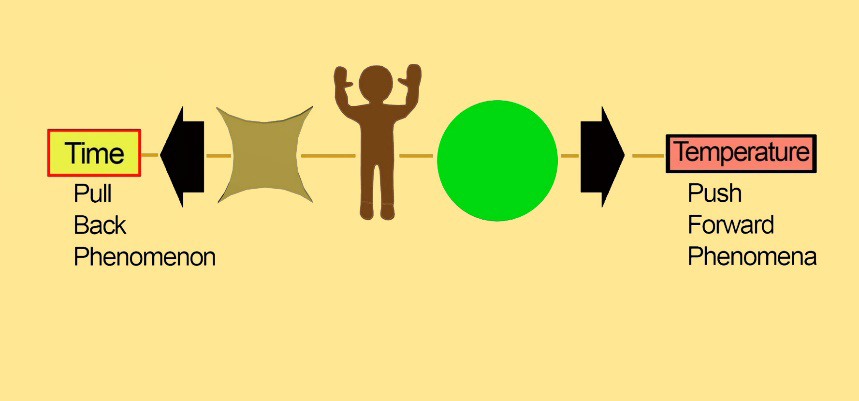
Until now the parameter time is being expressed as distance. Distance and time cannot be the same. Once the true definition of time is evolved, the significances of all the physical variables of the universe will turn out to be different.
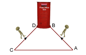
Time is related to the inter-molecular attractive forces or one may call “time” as a pull-back phenomena. In the Figure 6 above two persons are being shown and they are travelling in the same distance to reach to a post office box to drop letters. Now as per the real concept of time, if one of the persons is pulled back by some invisible force towards the origin and another person does move on its own without any such pull back, then the time required for the first person to drop the letter would be considered to be more than the other person. In fact, higher would be the pull back, higher would be the time requirement. In a matter, when the cohesive forces among the molecules are at their maximum level, the time reaches a value of infinity. This can be compared with the case of a ‘Black- Hole’. In a Black-Hole in its most compressed state, the time is infinity, but if the Black-Hole would have expanded and expanded, the time would have decreased and decreased exponentially and would be approaching zero ultimately. The concept of time could be built from an example of a football match. When a football match starts, the time in hand is say 90 minutes (conventional definition of time) and as the football match progresses, the time decreases and decreases, and becomes zero at the end of the match. The real concept of time is this. When the universe was born, the time was infinity (the molecular attractive forces were maximum). But as the universe is getting larger and larger the time is decreasing and decreasing.
The ‘time’ is a diminishing phenomenon with the expansion of the universe. ‘Time’ is a pullback force phenomena or inverse force phenomena. From the thermodynamic point of view, we defined time as, t = time = ( ) ( )
$$ - = \frac {3 \mathrm {r}}{4 \pi \mathrm {r} ^ {3}} = \frac {3}{4 \pi \mathrm {r} ^ {2}} $$ (12) The extent to which, the entropy is being pulled back by randomness or energy, is in fact the real ‘time’ variable of the universe. As r → o t→∞ As r →∞t→o On the other hand, “Temperature” is the inverse of time. Temperature is the real inverse of pull back phenomena or the push forward phenomena So, T = Temperature = Randomness or energy entropy (13) So ‘Temperature’ is the measure of “the extent to which randomness pushes forward the entropy”.
$$ : \frac {4 \pi r ^ {3}}{3 r} = \frac {4 \pi r ^ {2}}{3} \tag {14} $$
So T = temperature =
2 $$ \frac {3}{4 \pi r ^ {2}} \times \frac {4 \pi r ^ {2}}{3} = 1 \tag {15} $$
So Time x temperature =
So pressure = P=Tt = 1 (16)
Concept of Volume and Velocity
Velocity in fact is very much related to the volume. The question arises that how the velocity (conventional definition) be the volume Velocity = Distance time (17) In the current model, distance is an integral multiple of inter molecular distance and can be expressed in the form of r and time, we already has defined as (3/4πr2)
3
4 3 r $$ \frac {r}{3} = \frac {4 \pi r ^ {3}}{3} (1 8) $$
r So velocity (by conventional definition) =
2 3 4 π So velocity in fact takes the shape of volume when the actual definition of time is considered.
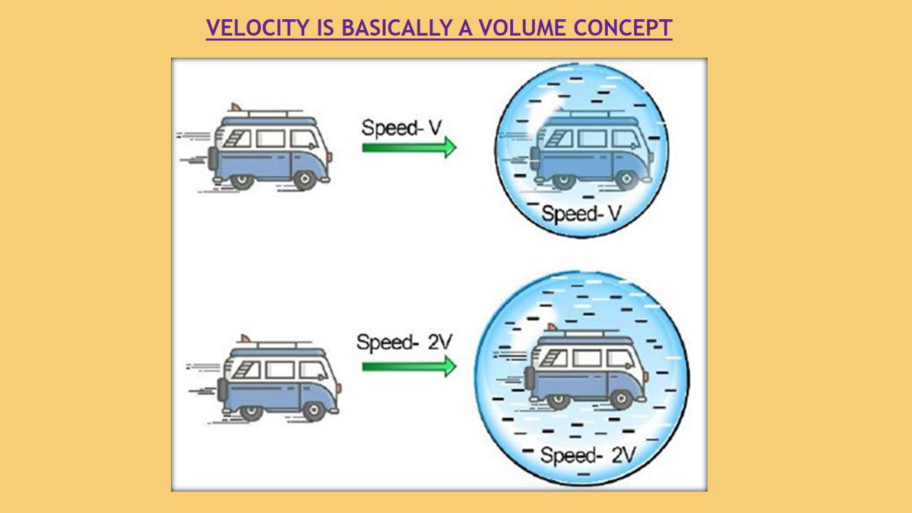
The moving vehicle (as shown in Figure 7 above) firstly has to overcome some or the other pull back force and then it makes an impact on the environment or space. The net result is the creation of a volume. At a first glance, the statement ‘Velocity is a concept of Volume’ sounds obscure but it is true. This concept of ‘time’ is explained below more explicitly in regard to the intermolecular attractive forces and rheology properties of matter.
The classical definition of Surface tension and viscosity
are:
Surface Tension of a liquid = (Force/Distance) = (Energy /
$$ \mathrm {A r e a}) = \left(\mathrm {L} ^ {2} \mathrm {M T} ^ {- 2}\right) / \mathrm {L} ^ {2} = \mathrm {M T} ^ {- 2} $$ Viscosity of a liquid = (Force/Area) x (Distance/Velocity) = $$ \left(\mathrm {L} ^ {2} \mathrm {M T} ^ {- 2}\right) $$
/(L2 x L/T) =
$$ = \left(\mathrm {M T} ^ {- 1}\right) / \mathrm {L} $$ So if the dimension of surface tension (ST) is being divided by the dimension of viscosity (VSC), one obtains (ST/VSC) = LT-1 The parameter LT¯¹ stands for the dimension of velocity. But what this velocity stands for has not been evaluated and is still an unanswered question in science. However, no satisfactory explanation could be put forward of this, ‘apparent look’ velocity dimension. The above said velocity dimension turns into a concept of ‘volume’ as is being shown below. Surface tension is a hybrid phenomenon of ‘order’ and ‘disorder’. While the ‘volume’ is a representation of ‘randomness’, the ‘intermolecular attractive forces’ is an index of ‘order’. The physical variables ‘volume’ and ‘intermolecular attractive forces’ are the responsible physical variables, those give rise to the phenomenon of ‘surface tension’. The surface tension can be expressed in the hybrid form as:
ST = (volume) x (intermolecular attractive forces) (19)
The viscosity of a liquid is directly related to the intermolecular attractive forces, the order creating physical variable. However, when one considers the flow of a liquid, the pressure is the actual physical variable which is responsible for flow. So viscosity is also another, ‘order- disorder’ hybrid phenomena. While the pressure imposes the ‘randomness’, the ‘intermolecular attractive forces’ try to retain the ‘order’. So viscosity in the hybrid form can be written as VSC = (pressure) x (intermolecular attractive forces) (20) ST and VSC, both are directly proportional to ‘intermolecular attractive forces’ but the former is linked to ‘volume’ and the latter is linked to ‘pressure’.
So, from the above discussion, one is led to conclude that, (ST/VSC) = (VOLUME) / (PRESSURE) (21) Now pressure is a dimensionless parameter (as has already been described in this article) and as a result the ratio of ST to VSC is a parameter which represents the dimension of ‘volume’. Now, if the classical definition of the ratio of ST to VSC is being compared with the TTQG definition, as just arrived above, one obtains the following relationship: (ST/VSC) = LT¯¹ = volume = L³ (22) So, T = time = (1/L²) (23) So the true dimension of ‘time’ is evolved. ‘Time’ is in fact an inverse force or an inverse area phenomenon of the universe.
Viscosity being the hybrid of molecular attractive force and pressure de-hybridizes surface tension (hybrid of molecular attractive force and volume) leaving behind the volume only as dimension, since pressure is dimensionless.
Two very important concepts do emerge from the above said exercise and those are: a. Time is an inverse force phenomena b. Velocity relates to volume when the actual dimension of time is taken into account.
Suppose in a vessel there exists a gaseous substance and it is under equilibrium with the surroundings at a constant pressure P=1 shown in Figure 8 below.
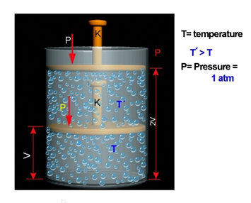
Suppose in a vessel there exists a gaseous substance and it is under equilibrium with the surroundings at a constant pressure P=1 shown in Figure 8 above.
If we increase the average velocity of the molecules by imparting energy in the system (by giving heat), the molecules get accelerated and under the equilibrium constant pressure condition the volume will go on increasing. If we go on supplying more heat in the system, the kinetic movement of the molecules will be higher and higher and the volume will also increase. If we extract out heat from the system the kinetic movements of the molecules will decrease and the volume will also decrease. So in fact velocity is truly a concept of volume rather than the directional displacements of the molecules of the system. In TTQG theory all the physical variables of the universe like, length, area, volume, energy, time, and temperature can be expressed in terms of intermolecular distances or the inverse of the intermolecular distances. So, all the physical variables are integral multiples of the intermolecular distances or the inverse of intermolecular distances. In other words this universe is integral with respect to all the physical variables and ‘fraction’ is simply a parameter which is of mathematical validity only and has no existence in reality. The main postulates of the unified quantum gravity (QG) theory of the universe can be summarized as under:
i) Inverting lengths (or inverting entropy gravitons) in all 3 principal directions form masses. ii) Expanding lengths (or entropy gravitons) in all the 3-principal direction generates volumes or energies. iii) This universe is an integral universe and originates from the disintegrations of the ‘SINGULARITY’ gravitons. The universe is integral in regard to principally, the entropy gravitons and the anti-entropic or order gravitons. iv) Gravitational field is basically an inverse acceleration field, originated from the mutually interacting astronomical bodies of the universe and the different types of gravitons are evolved from the said inverse acceleration fields. The acceleration field in turn, is linked to the intermolecular attractive forces. v) Gravitational constant G, as proposed by Sir Isaac Newton [76, 79, 81, 84, 85, 86, 87] is not a constant and is a variable of the universe and is a composite variable function of mass, distance of separation of two objects, the time and the forces acting between the two objects vi) The universe is formed by the translational motion of the entropy/order gravitons coupled with their rotations and twisting. Any geometrical or real object; one can draw from a point only (Figure 9) vii) Time is a pull-back phenomena and is an inverted circle which acts in opposition to the forward movement of the molecules. Time is a pull-back inverting phenomena as shown in (Figure 9)
viii) Temperature is a push forward phenomenon and is a circle too and which accelerates the forward movement of the molecules. ix) Time and temperature is just multiplicative inverse to each other. So the universe can be represented by a time- temperature mathematical equation t T = 1 x) There is no such variable as ‘velocity’ in the true sense. Velocity in fact is volume and the average volume increases with the average random motion of the molecules. The measure of average random motion of the molecules is ‘entropy’ but not velocity. There is no such thing in the nature as truly directional. Whatever we find or watch as a directional, ultimately it is converted to randomness. xi) All the 3 laws of motion of Sir Isaac Newton has got serious limitations, especially in a molecular level and that will be elaborated later. xii) Einstein’s equation, E = mc², relating mass (m), energy (E) and velocity of light (c), has also got serious limitation and is not at all a representation of true mass- energy equivalence of the universe.
Concept of Mass and Acceleration
We now derive the expression of acceleration and mass in terms of the intermolecular distance.
Acceleration by definition is the rate of change of velocity with time. Now velocity equates to volume, once the true definition of time is adopted.
So Acceleration =
4 16 3 3 9 4
3 2 5 π π r Velocity or Volume r time r $$ \frac {1}{2} = \frac {3 ^ {\pi 1}}{3} = \frac {1 6 \pi^ {2} \mathrm {r} ^ {5}}{9} \tag {24} $$
2 π So acceleration is a five dimensional entity and it represents how the volume changes with time.
To derive the expression of mass, we will use the fundamental equation of pressure and which is . . Pressure h g ρ = (25) h = height or depth ρ = density g = acceleration Now this can be shown simply as a product of push forward and pull back phenomena on rearranging.
Pressure P h g ρ = =
= Mass h x x acceleration Volume
= h x mass x acceleration Volume
= distance volume
x (mass x acceleration)The first part of the above equation, (distance/volume), can be compared to (entropy/randomness) or pull back and the second part is the push forward force. So Pressure = pull back force x push forward force For a matter in equilibrium with the surroundings, P =1. Now h here is the depth of the matter
3
4 3 3 4 π r volume r surface area r π = = = (26)
2
r
2 5 16 9 r π (27)
3 4 3 So, P = 1
$$ = \frac {(3)}{\left(\frac {4}{3} \pi \mathrm {r} ^ {3}\right)} $$
x m x
3 m = mass = 3 2 5 4 3 9 3 16
$$ \frac {4}{3} \pi r ^ {3} x \frac {3}{r} x \frac {9}{1 6 \pi^ {2} r ^ {5}} = \frac {9}{4 \pi r ^ {3}} \tag {28} $$ Now momentum = mass x volume $$ = \frac {9}{4 \pi r ^ {3}} x \frac {4}{3} \pi r ^ {3} $$
= 3 (29) So momentum is a constant and can be equated to 3. Energy (E) is, Force x distance $$ = 4 \pi r ^ {2} x r = 4 \pi r ^ {3} \tag {30} $$ Now mass x energy $$ = \frac {9}{4 \pi r ^ {3}} \mathrm {x} 4 \pi \mathrm {r} ^ {3} = 9. $$
Representation of the Principal Physical Variables in Regard to TTQG Theory in 2- and 3-Dimensions
Time, velocity, momentum, mass, acceleration, density entropy, force, energy can all be represented in this model in terms of r, in both 2- and 3-dimensions [1, 2, 3, 4, 5, 6, 7, 8, 9, 10, 11, 12, 13, 14, 15, 16, 17, 18, 19, 20, 21, 22]. This is shown in the following table.
| S. No. | Physical Variable | 2-dimension | 3-dimension |
|---|---|---|---|
| 1. | Depth of matter | Area/circumference = πr²/2πr = r/2 | Volume/surface area = 4/3πr³/4πr² = r/3 |
| 2. | Force | Pressure x circumference = 2πr x 1 = 2πr | Pressure x area = 4πr² x 1 = 4πr² |
| 3. | Energy | Force x distance = 2πr x r = 2πr² | Force x distance = 4πr² x r = 4πr³ |
| 4. | Entropy | 2r | 3r |
| 5. | Time | entropy/energy = 2r/2πr² = 1/πr | entropy/energy = 3r/4πr³ = 3/4πr² |
| 6. | Temperature | energy/entropy = πr²/2r = (πr/2) | energy/entropy = 4πr³/3r = (4/3πr²) |
Table 2: QG theory derived quantum units in 2- and 3-dimensioins of the principal physical variables of the universe.
- 7.
- Velocity distance r r time r
- 2
- 1 distance r r time r
- =
- =
- 3 π
- =
- = π π
- 8.
- Acceleration
- 2
- 2
- 3
- 1 r velo t r tim ci y e r π π r velocity r time r
- =
- =
- =
- = π
- 2 π
- 1=
- 2
- 3 depth of matter mass x r area π
- ×
- 9.
- Mass
- Mass =
- 3
- 9
- 4 r π
- 2
- 3
- 2
- 2 r mass r ðr π
- =
- ×
- ×
- ×
- 2
- 2
- 4
- 2
- 2
- 2 r r r π π π
- =
- Mass =
- 10.
- Momentum
- Mass x volume=
- 2
- 2
- 2
- 2 x r r π π
- =
- =
- 3
- 3
- 9
- 4
- 3
- 4 x r r π π
- = 3
- 3
- 4
- 4
- 3
- 3
- Mass r
- Volume r π
- 2
- 2
- 2
- Mass r
- Volume r area r
-
-
-
-
-
-
- =
- =
- =
- 3
- 2 π π π
- 11.
- Density
- (
- )
- (
- )
- (
- )
- 2
- 2
- 2
- 2
- 2
- 3
- V
- (V= Volume)
Table 3: QG theory derived quantum units in 2- and 3-dimensioins of the principal physical variables of the universe.
The 4 very important equations derived in TTQG, mv = 3 (31) Tt = 1 (32) mE = 9 (33) E = 3V (34)
Origin of Gravitation
Gravitation [25, 26, 27, 28, 29, 30, 31, 32, 33, 34, 35, 36, 37, 38, 39, 40, 41, 42, 43, 44, 45, 46, 47, 48, 49, 50, 51, 52, 53, 54, 55, 56, 57, 58, 59, 60, 61, 62, 63, 64, 65, 66, 67, 68, 69, 70, 71, 72, 73, 74, 75, 76, 77, 78, 79, 80] is in fact, originated from molecular attractive forces or Van der Wall’s forces. Lei Zhang [3] had given a very logical explanation of this spread of Van der Wall’s forces up to a very large distance, in his article, entitled “The Van der Walls force and gravitational force in matter”. If one considers a heavy astronomical object, in it, the innumerable infinitesimal Van der Walls force fields do overlap and converge, on an average, to a single, integrated and high magnitude attractive force field. This said, high magnitude attractive force field acts as some squeezing force, acting on the other astronomical object situated at a certain distance from the first heavy astronomical object. As a result of this, the second astronomical object, experiences, a squeezing or an inverse acceleration. So an inverse acceleration field is evolved from the center of Mass of the second astronomical object. The second astronomical object, in a similar fashion, imparts a squeezing force on the first astronomical object and another inverse or squeezing acceleration field is also evolved from the center of mass of the first astronomical object. So ‘Gravitation’ being a tangible physical variable, can be viewed as an overlapping field of 2 nos. of mutually interacting inverse accelerations, as explained above. Gravitation being the most important phenomenon of the universe can be defined also as ‘diminishing, but infinitely spread Van der Walls force field in space’ (see Figure 10).
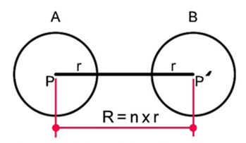
Suppose there are two number of masses of radius r and are situated at a distance R (= nr, n is an integer) from each other as shown in Figure 11 above Gravitation is in fact, is originated from molecular attractive forces. The molecules of A attract the molecules of B and molecules of B attract the molecules of A. So both A and B go under some accelerating. As a matter of fact the two accelerators fields overlap with each other and the gravitational force field do generate. The result of such overlapping may be called as an overlapping of two numbers of inverse acceleration fields and can be represented as:
2 5 2 5 9 9 16 16 x r r π π (35)
So, if acceleration is represented by f then gravitation in the form of super ‘graviton’ or ‘singularity’ (to be elaborated later) being a pullback phenomenon will be, Super Graviton or Super entropic Graviton or Singularity = (inverse acceleration)2 $$ = \frac {1}{f ^ {2}} \tag {36} $$ Why this is called ‘super graviton’ or ‘super entropic Graviton’ or a ‘Singularity’ and how a ‘Super graviton’ step-by-step transforms to entropy and what in fact is the phenomenon of an ‘entropy to entropy’ flight of the super graviton, has been discussed.
However, the dimensionality of the super graviton is 10,
Now as per Newton’s law of gravitation for two masses (each is of radius r) separated by a distance R the gravitational constant G can be equated to as shown below
2
2 R x force R nr m = (37)
G = [ ]
Here n is a integral multiple of the entropy, r If the dimensions force and mass are put in the above equation, the Newton’s Gravitational constant become
2 2 3 10
4 16 81 9 4 π π r x r r G x n n x = ( ) 2 4 n x acceleration π $$ G = \frac {r ^ {2} x 4 \pi r ^ {2}}{\left(\frac {9}{4 \pi r ^ {3}}\right) ^ {2}} x n = r $$
2
3 π r (38) Gravitational constant of Newton = 2 . 4 n f π (39)
So Gravitational constant of Newton was an obscure entity in the form of Newton kg-2m2 but the present theory explores it in the form of distinctly dimensionally understood physical variable as (acceleration)2. Newton’s gravitational constant is placed, however, in the reverse sense than what gravitation is in reality and that will be proved now.
The dimension of gravitational constant (G) can be written as (from equation 37): G = Gravitational constant of Newton = (Force x Area)/(Mass x Mass) $$ = \left(\mathrm {L M T} ^ {- 2}\right) \mathrm {L} ^ {2} / \mathrm {M} ^ {2} = \mathrm {T} ^ {- 2} \mathrm {L} ^ {3} / \mathrm {M} $$ So, G x (M/L3) x T2 = 1.00 (40) Since (M/L3) has a dimension of density, one can write, G x Density x T2 = 1.00 (41)
G can also be written in the other form as, G = (Mass x acceleration x distance x distance)/(Mass X Mass) Or, G = (acceleration x distance x distance)/(mass) Or, G = (Acceleration xL2)/M Or, G x mass x (1/ acceleration) x ( 1/L2 ) = 1.00 (42) As per equation (42), one can take masses of any magnitude of desire, place them at any distance and can vary the acceleration as per his own choice. As a result the term, mass x (1/ acceleration) x (1/L2), can never be a constant. So, if G is considered to be a constant, the equation (42) will never give a result of unity. So G has to attain different values to make equation (42), valid. So the Newton’s Gravitational constant cannot be considered to be a constant at all.
Again, as it is found from equation (41), for a fixed value of time, T, the densities can have many values. On the contrary for a fixed density, the time T, can have different values. So again G, ceases to be a constant since if G is a constant and (Density x T2) have different values, Equation (41) will not be a valid equation. So the magnitude of G has to vary and has to vary in a fashion such that the magnitude of G and (Density x T2) has to be multiplicative inverse to each other and the value of equation (41) is always being unity.
A very strong evidence that G does not represent the phenomenon of Gravitation in the proper sense is revealed from the following exercises: Equation (37) is:
So when m→∞, G→0 and when m→0, G→∞ In the event of masses being enormously higher, the gravitational pull should be pretty high in magnitude and when the masses are vanishingly small, the pull - back force should be very feeble. However, the pattern of G as per equation (37) just reflects the reverse picture.
If we define a function G′ and which is equal to (1/G), then we get the proper representation of Gravitation, then equation (37) transforms to :
When m→∞, G′→∞ and when m→0, G′→0. This is in conformity with the phenomenon of gravitation. So Newton’s Gravitation theory suffers from the following two numbers of serious limitations: 1. The Gravitational constant G as defined by Newton is not a constant and is a variable physical parameter of the universe and is a function of time. 2. Presenting gravitation in the form of ‘G’, does not truly represent the phenomenon of gravitation. In fact the inverse of the function G, represents the gravitation phenomenon properly. G in Newton’s law is being placed in the reverse fashion than what ‘gravitation’ is. The same logic applies to the Hubble’s constant.
The Hubble’s law is expressed as [75]
V = Ho D (44) Where Ho is constant of proportionality and D is the distance of a galaxy. Ho = V/D = Hubble’s constant For a fixed value of D, the velocities can have different values. Also for a fixed value of velocity, the distance can have many values. So Ho cannot acquire any constant value at all
| S. No. | Dimensions | Description |
|---|---|---|
| 1 | r | Distance, entropy, potential difference |
| 2 | r2 | Force, push forward, temperature, charge |
| 3 | r³ | Energy/volume, intensity, conductance |
| 4 | r4 | EM wave, electrical current |
| 5 | r⁵ | Acceleration, power |
| 6 | r⁶ | Photo electricity |
| 7 | r⁷ | Nuclear fission |
| 8 | r⁸ | X-rays |
| 9 | rꝰ | Plasma state |
Table 4: TTQG Depicted Dimensions of Several Gravitons.
Principle Concepts Of TTQG: Schematic Presentations
In this section of the research article, some principle concepts of TTQG are presented schematically. Before that the following points are to be noted: 1. Max Planck tied up the five numbers of basic physical variables of the universe (Length L, Mass M, Time T, Temperature and Electric Charge) to the same source in terms of the Newton’s Gravitational Constant ( G) and the Planck constant (h)[7]
2. Since the topologies of G and h were not known, the relation between L, M & T could not be established at that point of time of Max Planck.
3. Later on, the quantum physics, QP [4, 5, 27, 28, 29, 30], could not erase the stamp of abstractness of the above said physical variables. QP also failed to evaluate the physics underlying the phenomena of gravitation, dimension of electromagnetic wave and the topology of a ‘photon’ [5, 6, 7, 8, 9, 10, 11, 12, 13, 14, 15, 16, 17, 18, 19, 20, 21, 22, 23, 24, 25, 26, 27, 28, 29, 30, 31, 32, 33, 34, 35, 36, 37, 38, 39, 40, 41, 42, 43, 44, 45, 46, 47, 48, 49, 50, 51, 52, 53, 54, 55, 56, 57, 58, 59, 60, 61, 62, 63, 64, 65, 66, 67, 68, 69, 70, 71, 72, 73, 74, 75, 76, 77, 78, 79, 80, 81, 82, 83, 84, 85, 86, 87, 88, 89, 90, 91, 92, 93, 94, 95].
| S. No. | Name of variable | Dimension | Expression | TTQG derived dimensions of the physical variables |
|---|---|---|---|---|
| 1 | Planck length | Length(L) | G = p c3 | r |
| 2 | Planck mass | Mass(M) | m= hc /G | 1/r³ |
| 3 | Planck time | Time(T) | G t = p c5 | 1/r² |
| 4 | Planck charge | Electric charge(Q) | q 4π p = oc | r² |
| 5 | Planck temperature | Temperature (θ) | c5 T = p Gk2 B | r² |
Table 5: Dimensions of Planck units of Length, mass, Time, charge and Temperature.
TTQG has evaluated all the above and introduced the following altogether new concepts in physics.
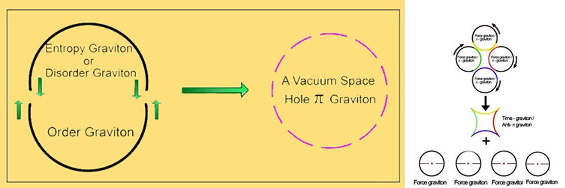
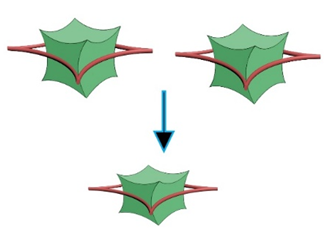
Figure 13a: Formation of ‘Time’ Graviton from the closely interacting of 4 nos. of ‘Force Gravitons’. The direction of rotation of the force gravitons are shown by arrow. On the figure, the similar fashion an anti-π graviton is formed from 4 nos. of rotating π gravitons.
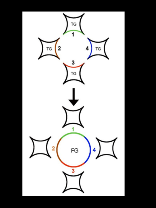
Figure 13b: Formation of a Force Graviton (FG) from 4 nos. of Time Gravitons (TG) or formation of a π Gravitons from 4 nos. of anti-π Gravitons.
Reformulation of Newtonian Physics, Through the Concept of TTQG.
Newton’s law of motions is based on macroscopic observations on the movement of objects. The connection of movement of the objects to the ‘space-time’ [4, 31, 32, 33, 47, 59, 77] was fully ignored. The physical variable ‘acceleration’ is an ambiguous physical variable since it suffers from the problem of ‘circularity of definition’ as shown in Figure 14 below:
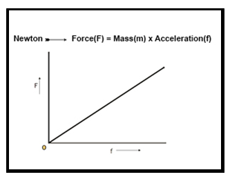
![Figure 15: Mass and Space expansion (Acceleration) interaction to produce force. The outer circle of the sphere in figure.15 is stretching the sphere and as a result there is a ‘space expansion’. So ‘acceleration’ of NP is ‘space expansion’ in TTQG and ‘inverse acceleration’ of NP is ‘space inversion’ in TTQG. So, one can write, SPACE EXPANSION =( FORCE / MASS), SPACE INVERSION = (MASS / FORCE) As per Newtonian Physics [84], when the mass, m, is constant, the plot of Force( F) versus acceleration(f) will give a straight line passing through the origin as shown in Figure 16 below. So as per NP, both force and acceleration are boundless variables of the universe. This cannot be true since this will violate the concept of ‘conservation of mass and energy’.](/fulltextimages/9831/fig_15.png)
However, velocity and time are related to each other. This is called ‘circularity of definition’ and is a major short-fall of Newtonian Physics. As per TTQG, ‘acceleration’ is a ‘space expansion’ phenomenon as shown in Figure 15.
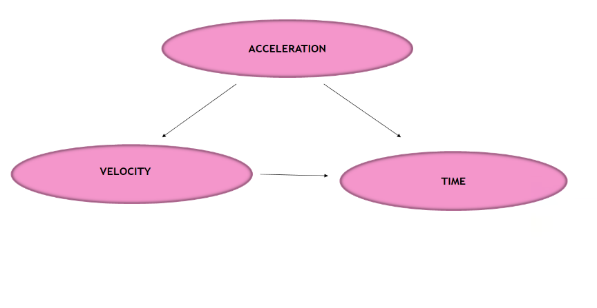
Figure 15: Mass and Space expansion (Acceleration) interaction to produce force. The outer circle of the sphere in figure.15 is stretching the sphere and as a result there is a ‘space expansion’. So ‘acceleration’ of NP is ‘space expansion’ in TTQG and ‘inverse acceleration’ of NP is ‘space inversion’ in TTQG. So, one can write, SPACE EXPANSION =( FORCE / MASS), SPACE INVERSION = (MASS / FORCE) As per Newtonian Physics [84], when the mass, m, is constant, the plot of Force( F) versus acceleration(f) will give a straight line passing through the origin as shown in Figure 16 below. So as per NP, both force and acceleration are boundless variables of the universe. This cannot be true since this will violate the concept of ‘conservation of mass and energy’.
In Figure 17a & 17b, the TTQG derived topologies of ‘Force’ and ‘Time’ are represented. From the said Figures and the mathematics involved there one can conclude that 1. ‘Force’ is the ‘geometric mean’ of ‘space expansion’ and ‘degree of order’. 2. ‘Time’ is the ‘geometric mean’ of ‘space inversion’ and ‘degree of randomness or entropy’ So TTQG very firmly establishes the fact that neither the ‘force’ nor the ‘Time’ are boundless. In fact both the said variables are very much bounded. When ‘Force’ tries to take higher and higher values, the degree of order is pulling it back such that it cannot attain an infinite magnitude. On the contrary, ‘Time’ being a ‘squeezing or attractive physical variable’ cannot become too squeezing since the ‘entropy’ will push it forward.
Figure 17a: Topological representation of ‘force’.
Figure 17b: Topological representation of ‘time’.
General Theory of Relativity Merging to Entropic Gravity of TTQG
Einstein field equation (EFE) of general relativity [31, 32, 33, 34] is bit mathematical and obscure, but the Einstein field equation conceptually represent the ultimate ‘left out state’ of the phenomena of gravitation, after all the physical variables play their roles and interact among themselves. Unified theory reveals that the EFE is dimensionally the same as entropy.
Before doing this exercise, we will examine what is ‘Gravitational force’ and ‘gravitational constant’ are, in regard to Newton’s law of Gravitation.
Gravitational Force = F = 1 2 2 . m m G r
(45) Now, if we dimensionally analyze this
1 r r = G.t4 = G.S-8 (46)
6 Gravitational force = G x
2 The Gravitational constant, on the other hand is G = Gravitational force x r8 = Gravitational force x t-8 = Gravitational force x S8 (47) So gravitational constant of Newton is super intense entropy gravitational force. This super intense entropic gravitation falls down to the super weak entropic gravitation once the super/singularity ‘GRAVITATON’ is fully unfolded.
Einstein field equation is
$$ R _ {\mu v} - \frac {1}{2} R ^ {2} g _ {\mu v} + \Lambda g _ {\mu v} = \frac {8 \pi G}{C ^ {4}}. T _ {\mu v} $$ (48) v Rµ - Ricci curvature tensor R – Scalar curvature v Gµ - Metric tensor Λ – Cosmological constant G – Newton’s gravitational constant C – Speed of light ì v T - Stress energy-momentum tensor Now if we analyze the dimensionally of the r.h.s of Equation (48), we get the following
10
4 4 2 3 8 1 81 8 1 256 4 C x r r
x x (81/256) (49) G xr
π π $$ \frac {1}{2} = \left(\frac {1}{2 5 6}\right) x \frac {8 1 x 8 \pi x r ^ {1 0}}{\left(r ^ {3}\right) ^ {4} x 4 \pi} = \frac {1}{2} $$ ( ) x π And v µ T = stress x energy x momentum $$ = \frac {r ^ {2}}{r ^ {2}} x r ^ {3} x 3 = 3 r ^ {3} \tag {50} $$ $$ = \frac {F o r c e}{a r e a} x r ^ {3} x 3 $$
Force x r x
area = So combining the (8πG/C4) part and v µ T part, the net dimensionality turns out to be $$ \frac {1}{r ^ {2}} x 3 r ^ {3} x \left(\frac {8 1}{2 5 6}\right) = \left(\frac {2 4 3}{2 5 6}\right) r \tag {51} $$ EFE ultimately merges to the entropy dimensionality of the universe and this is in full agreement with the observation made by Edwin Hubble [35, 36, 37, 38] that the universe is expanding since entropies are being generated.
Special Theory of Relativity and TTQG
The special theory of relativity [78] has offered an ‘energy-mass’ equivalence equation in the form of E = mc² [E=Energy, m=mass, c=velocity of light] The above equation is not acceptable due to the following reasons:
- When mass is zero, energy is also zero. When mass in infinity, energy is also infinity. This is not true since neither the mass nor the energy of the universe can take zero or infinite values.
- The dimensions of mass, time, and energy not presented by Albert Einstein while proposing the above equation.
- In the said equation of Einstein, if one plots E verses m, it will give a straight line passing through the origin.
This means that mass and energy both simultaneously go towards infinite magnitude. This is fully violating the ‘laws of conservation of mass and energy’ of the universe. This is also in total contradiction with the current concepts of Cosmology where in a Black-Hole the mass is infinite and energy is approaching zero.
If the Einstein’s energy-mass equivalence equation is being examined by the philosophy and logic of TTQG, it can be rewritten in the following form: E = mc x c (52) The parameter C in the above equation (15.1) is a velocity parameter and in TTQG velocity is a concept of volume (V) as has been clearly demonstrated in TTQG [98, 99, 100, 101, 102].
So, the above equation can be rewritten as in terms of volume: E = mV x V …….. (53) As per TTQG, mV = momentum = 3, and so, the above equation takes the form E= 3V This has been already shown at the beginning of this article and this is the ‘actual energy-space’ representation of the universe. However, Einstein did arrive to an improper representation of energy in the form, E = mc², without considering the i) topology and dimensionality of the physical variables and the ii) the universal graviton cycle of the universe respectively.
Summary and Conclusion
All the research findings (as described above) of this article are based on the principle philosophy of TTQG viz.: ‘DIMENSIONALITY OF VOLUME AND ENERGY ARE THE SAME’. Dimension of energy = ML²T¯² Dimension of volume = L³. So, when above said dimensionalities are compared to each other, one gets ML²T¯² = L³ Or, MT¯² = L Or, (Mass) = (Length) x (Time) ² Or, (Time) = (Mass x Degree of Order) ½ [ (Mass) = 1/ ( Volume), Degree of order = (1/ L) ]
So, connecting Mass (M), Time (T) & Length (L) through the above equilibrium (MT¯²=L), TTQG solved the following cosmic mysteries of the universe [50, 53, 58, 60, 90, 91, 92, 93, 94, 95, 96, 97].
- The dimensionality of ‘time’, ‘mass’, phenomenon of ‘gravitation’ and the ‘universe’ have been evaluated. The labels of abstractness on the above said variables have been totally removed.
- The ‘conservation of momentum’, ‘time-temperature inverse equilibrium relationship’ and ‘mass - energy or volume equilibrium’ has been established from the angle of equilibrium topologies of ‘π graviton- anti π graviton’ or ‘force graviton- time graviton’.
- The phenomenon of ‘Black Body radiation’ explained on the basis of the actual dimension of ‘spectral power distribution’.
- Dimension of ‘nuclear fission’, ‘nuclear fusion’, ‘black- holes’ and ‘plasma state’ have been evaluated.
- ‘Cold nuclear fusion phenomena’ has been proved to be a real phenomenon of the universe and not an ‘experimental artifact’.
- The two different branches of physical science, viz, i) quantum physics and ii) TTQG unified to each other.
- The phenomenon of ‘mass defect’ explained in regard to ‘entropy graviton’
- New theory of color physics (TTQG theory of color) discovered which explained for the first time the origin of 7 colors of VIBGYOR, cosmological red shift, Sun’s energy spectrum, etc and others.
A new ‘UNIVERSAL GRAVITON CYCLE MODEL’ model has been presented in TTQG. The said model is originated from ‘SINGULARITY GRAVITON’ and the cycle reveals all the natural or cosmic phenomenon of the universe as shown in Figure 18 below:
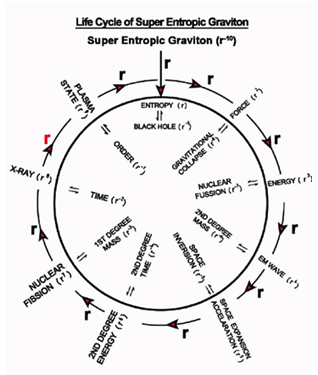
Table 5 below shows the different steps by which a singularity graviton gradually decays to evolve the multi various dimensions and natural or cosmic phenomenon of the universe.
| Step No. | State of Graviton | Emission From the Graviton | Equilibrium between Push Forward and Pull Back Gravitons | Observable Physical Variables in Equilibrium with Each Other |
|---|---|---|---|---|
| 1 | 1 81 = f2 256π4 r10 | π | 81 ⇋ π 256π3 r10 | Empty space π-graviton and super entropic or singularity graviton |
| 2 | 81 256π3 r10 | r | 81 ⇋ π r 256π3r9 | Entropy graviton and Black-hole graviton |
| 3 | 81 256π3r9 | r | 27 4 ⇋ πr2 64π3r8 3 | Fourth degree time graviton and push forward / temperature/force graviton |
| 4 | 27 64π3r8 | r | 81 ⇋ 4π r3 64π3r7 | Nuclear fusion graviton and first degree energy graviton |
| 5 | 81 64π3r7 | π r | 81 ⇋16π2 r4 16π2r6 | EM-wave graviton and 2nd degree mass graviton |
| 6 | 81 16π2r6 | r | 9 16π2r5 ⇋ 16π2r5 9 | Space inversion-space expansion, color graviton of object,and color graviton of EM wave |
| 7 | 9 16π2r5 | r | 9 16π2r6 ⇋ 16π2r4 9 | 2nd order time graviton or 2nd order force or temperature graviton |
| 8 | 9 16π2r4 | π r | 9 64π3r7 ⇋ 4π2r3 9 | 1st order mass and nuclear fission graviton |
| 9 | 1 4π r3 | r | 3 64π3r8 ⇋ 4πr2 27 | Time graviton and X-ray, gamma ray graviton |
| 10 | 3 4π r2 | r | 1 256π3r9 ⇋ πr 81 | Plasma state graviton and order graviton |
| 11 | 1 πr | π | 1 ⇋ π r | Order graviton and π graviton |
| 12 | 1 | r | 1⇋πr | Enlarged singularity and entropy graviton |
Table 6: Decay of ‘singularity gravitons’ and evolution of multi various cosmic equilibrium of the universe.
So this research article very definitively establishes for the first time in physics the equilibrium relationship between L, M & T in the form, MT¯² = L
References
-
Jones JE (1924) On the determination of molecular fields. Proceedings of the Royal Society of London 106(738): 463-477.
-
Lim TC (2003) The relationship between Lenard Jones (12-6) and Morse Potential. Zeitschrift für Naturforschung A 58(11): 615-617.
-
Zhang L (2013) The Van der Waals force and gravitation force in matter. Physics gen ph, arXiv, 1303.3579.
-
Bonneville R (2016) An alternative model of particle physics in a 10-dimension (pseudo) Euclidian space time. High Energy Physics, arXiv.
-
Menon KK, Quarashi T (2017) Wave particle Duality in asymmetric Beam interference. Phys Rev A 98: 022130.
-
Zslavski OB (2005) Ultimate gravitational mass defect. Gen Rel Grav 38(5): 945-951.
-
Bolotin YUL, Yanoksky VV (2017) Modified Planck units. General Physics, arXiv.
-
Paul GH (2009) Maxwell’s equation.1st(Edn.), Wiley- IEEE Press, New Jersey.
-
Jackson JD (1998) Classical Electrodynamics. 3rd(Edn.), Wiley, New York, pp: 832.
-
Fundamental Physical Constant- Extensive Listing.
-
Halliday, Resnick (1974) 6 Power Fundamental of Physics. Vol 1, The Feynman Lecture on Physics.
-
Loudon R (2000) The quantum theory of light. 3rd(Edn.), Oxford University Press, UK.
-
Duffin W (1990) Electricity and Magnetism. 4th(Edn.), McGraw-Hill Education, Middle East & Africa, pp: 496.
-
Serway RA, Jewett JW, Wilson K, Wilson A, Rowlands W (2016) Physics for Global Scientists and Engineers. 2nd(Edn.), Vol 2, Cengage, pp: 901.
-
The NIST reference on fundamental physical constants.
-
Rybicki GB, Lightman AP (1979) Radiative Processes in Astrophysics. John Wiley & Sons, New York, United States, pp: 325.
-
Mcquarrie DA, Simon JD (1979) Physical Chemistry: A molecular approach. 1st(Edn.), University Science Books, Sausalito, USA.
-
Michael B (2013) Physics for Engineering and Science. 2nd(Edn) McGraw-Hill Education, New York, pp: 427.
-
Rybicki GB, Lightman AP (1979) Fundamentals of Radiative Transfer. In: Radiative Processes in Astrophysics. John Wiley & Sons, New York, United States, pp: 20-28.
-
Purcell ME, David J (2013) Electrical energy in a crystal lattice. In: Electricity and Magnetism. 3rd(Edn.), Cambridge University Press, New York, Cambridge, pp: 14-20.
-
Maxwell JC (1873) Treatise on Electricity and Magnetism. Vol 2, Oxford Clarendon Press, United States, pp: 236- 237.
-
The Nobel Prize in Physics 1921.
-
Arore MG, Singh M (1994) Nuclear Chemistry. Anmol Publications, Daryaganj, New Delhi, pp: 476.
-
Goldston RJ, Rutherford PH (1995) Introduction to Plasma Physics, Institute of Physics Publishing, Bristol, UK, pp: 479.
-
Sharma KS (2008) Atomic and Nuclear Physics. Pearson Education India, Dorling Kindersley, London, United Kingdom, pp: 620.
-
Verdenne G, Attetia JL (2009) Gamma-ray Bursts: The brightest explosions in the Universe. 1st(Edn.), Springer Berlin, Heidelberg, pp: 580.
-
Schrodinger E (1926) An undulatory theory of the mechanics of atoms and molecules. Phys Rev 28(6): 1049-1070.
-
Griffiths JD (2004) Introduction to Quantum Mechanics. 2nd ( Edn.), Prentice Hall, New Jersey, pp: 409.
-
Atkins PW (1977) Molecular Quantum Mechanics Parts I and II: An Introduction to Quantum Chemistry. Oxford University Press, United Kingdom.
-
Atkins PW (1974) Quanta: A Hand book of concepts. Oxford University Press, pp: 316.
-
Einstein A (1916) The foundation of the General Theory of Relativity. Annalen Phys 354(7): 769-822.
-
Grøn O, Hervik S (2007) Einstein General Theory of Relativity: with modern application is cosmology. 1st(Edn.), Springer, pp: 180.
-
Lemkhl D (2018) General Relativity as a Hybrid Theory: The Genesis of Einstein’s work on the problem of motion. General Relativity and Quantum Cosmology, arXiv.
-
Hess PO (2016) The Black Hole merger event GW150914 within a modified Theory of General Relativity. Monthly Notices of the Royal Astronomical Society 462(3): 3026- 3030.
-
Chrimes AA, Levan AJ, Stanway ER, Lyman JD, Fruchter AS, et al. (2019) Chandra and Hubble Space Telescope Observation of dark Gamma-ray bursts and their host galaxies. Monthly Notices of the Royal Astronomical Society 486(3): 3105-3117.
-
Bergh SVD (2011) The curious case of Lemaitre’s equation no. 24. J Royal Astronomical Soc of Canada 105(4): 151.
-
Nussbaumer H, Bieri L (2011) Who discovered the expanding universe. The observatory 131(6): 394-398.
-
Way MJ (2013) Dimantling Hubble’s Legacy? American Astronomical Society 471: 97-132.
-
Wald RM (1984) General Relativity. The University of Chicago Press, Chicago and London, USA.
-
Wald RM (1999) Gravitational Collapse and Cosmic Censorship. In: Iyer BR (Eds.), Black Holes, Gravitational Radiation and the Universe. Vol 100, Fundamental Theories of Physics, Springer, pp: 69-86.
-
Overbye D (2015) Black Hole Hunters. NASA.
-
Montogomey C, Orchiston W, Whittinghan l (2009) Michell Laplace and the origin of the Black-Hole Concept. J Astronomical History and Heritage 12(2): 90-96.
-
Abbott BP, Abbott R, Abbott TD, Abernathy MR, Acernese F, et al (2016) Observation of Gravitational waves from a binary Black Hole merger. Phys Rev Lett 116(6): 061102.
-
Telescope EH, Kazunori A**_,_** Antxon A, Walter A, Keiichi A, et al. (2019) First M87 Event Horizon Telescope Results. I. The Shadow of the supermassive Black-Holl. The Astrophysical J 875(1): 1-17.
-
Shapiro SL, Teukolsky SA (1983) Black Holes, White dwarfs and neutron star: the physics of compact objects. John Wiley and Sons, pp: 357.
-
(2017) Introduction to Black Holes.
-
Singh J (1995) Space Time Waltz. 1st(Edn.), Wiley Eastern Ltd, New Delhi, India, pp: 156.
-
Penrose R (2002) Gravitational Collapse: The Role of General Relativity. Gen Re Grav 34(7): 1141-1165.
-
Rose C (2013) A conversation with Dr. Stephen Hazking and Lucy Hawking.
-
Srikanta P (2017) Recent Development in intelligent Nature-Inspired Computing-Advances in Computational Intelligence and Robotics. Waterstones, pp: 264.
-
Giddings SB, Thomas S (2002) High energy colliders as black hole factories: The end of short distance physics. Physical Review D 65(5): 056010.
-
Belgiorno F, Cacciatori SL, Clerici M, Gorini V, Ortenzi G, et al. (2010) Hawking radiation from ultrashort lesser pulse filaments. Phys Rev Lett 105(20): 203901.
-
Grossman L (2010) Ultrafast laser pulse makes Desktop Black-Hole glow.
-
Kumar KNP, Kiranagi BS, Bagewadi CS (2012) Hawking Radiation: An augmentation attriton Model. Adv Nat Sci 5(2): 14-33.
-
Wilt BSD (1980) Quantum gravity: the new synthesis. In: Hawking S (Eds.), General relativity; An Einstein centenary. Cambridge University Press, UK, pp: 696.
-
Jacob DB (2008) Bekenstein Bound. Scholrapedia 3(10): 7374.
-
Hawking SW, Elliz GFR (1973) The large scale structure of space time. Cambridge University Press, UK.
-
Charles M, Jhorne Kip S, Wheeler J (1973) Gravitation. W.H.Freeman and Company.
-
Peacock JA (1999) Cosmological Physics. Cambridge University Press, UK.
-
Dieter B (2012) Black-Hole Horizons and How they begin. The Astronomical Review 7(1): 25-35.
-
Chen Y, Shu J, Xue X, Yuan Q, Zhao Y (2019) Proting Axions with event Horizon Telescope Polarimetric measurements. Physical Review Letters 124: 061102.
-
Giddings SB (2019) Searching for quantum Black-Hole structure with event Horizon Telescope. Universe 5(9).
-
Kunter ML (2003) Astronomy: A Physical perspective. Cambridge Univ Press, UK, pp: 148.
-
Schwarzschild K (1916) On the gravitational field of a mass point according to Einstein’s theory. Math Phys 189-196.
-
Robert W (1984) General Relativity. The University of Chicago Press, USA, pp: 152-153.
-
Simon S (1979) John Mitchell and Black Holes. Journal of the History of Astronomy 10: 42-43.
-
Dimitar V (2012) Consequence from conservation of total density of the universe during the expansion. Aerospace Res Bulg 24: 60-66.
-
McCornell NJ, Ma CP, Gebhardt K, Wright SA, Murphy JD, et al. (2011) Two ten billion solar mass black holes at the center of giant elliptical galaxies. Nature 480(7376): 215-218.
-
Sandesses RH (2013) Revealing the heart of the Galaxy The Milky Way and its Black-Hole. In: Sandesses RH (Ed.), Cambridge University Press, UK, pp: 36.
-
Carol SM (2004) Space-time and Geometry: An Introduction to General Relativity. In: Carol SM (Ed.), Cambridge University Press, UK.
-
Penrose R (1965) Gravitational collapse and space-time singularities Physical Review Letters 14(3): 57-59.
-
Kerr RP (1963) Gravitational Field of a spinning mass as an example of Algebraically Special Metrics. Physical Review Letters 11(5): 237-238.
-
Newman ET, Janis AI (1965) Note on the ker-spinning Particle Metric. Journal of Mathematical Physics 6(6): 915.
-
NASA (2018) Black Holes.
-
IAU (2018) IAU members vote to recommend renaming Hubble law as Hubble-Lemaitre law.
-
Haranas I, Gkigkitzis I (2014) The Mass Graviton and its relation to the number of information according to Holographic principle. International Scholarly Research Notices, 718251.
-
Benincasa P (2018) From the Flat Space S-matrix to the wave function of the universe. High Energy Physics- Theory, arXiv.
-
Modestino G (2016) Explanation of the Special Theory of Relativity by Analytical Geometry and Reformulation of the inverse square law. General Physics, arXiv.
-
Corichi A, Diag-Polo J, Borza EF (20007) Loop quantum gravity and Planck-size Black Hole entropy. J Phys Conf Ser 68: 012031.
-
Bojowald M (2007) Singularities and quantum Gravity. AIP Conf Proc 910: 294-733.
-
Ashtekar A (2007) An introduction to Loop Quantum Gravity through cosmology. Nuovo Cim B 122: 135-155.
-
Fan YZ, Wei DM, Xu D (2007) Gamma-ray Burst UV/ optical afterglow polarimetry as a probe of quantum gravity. Mon Not Roy Astron Soc 376(2007): 1857-1860.
-
Bojowald M (2007) Quantum gravity and cosmological observations. AIP Conf Proc 917: 130-137.
-
Hansson J (2010) Newtonian Quantum Gravity. Phys Essays 23: 53.
-
Ward BFL (2008) Resummed Quantum Gravity. Int J Mod Phys 17: 627-633.
-
Wamg CHT (2006) New ‘Phase’ of quantum gravity. Phil Trans Roy Soc Lond 364: 3375-3388.
-
Demir DA, Tanyildizi SH (2006) Higher curvature Quantum gravity and Large extra Dimensions. Phys Lett 633: 368-374
-
Kiefer C (2005) Quantum: General Introduction and Recent Developments. Annalen Phys 15: 129-148.
-
Lewis PA, Patton TC (1998) Pigment Handbook. In: Lewis PA (Ed.), Color Theory; Characterization and Physical Relationships. 2nd(Edn.), Vol 3, Wiley, pp: 229-288.
-
Zones FN, Nichols ME, Pappas SP (2007) Orgnic Coatings: Science and Technology. In: Wicks ZW (Ed.), Organic Coatings. 4th(Edn.), Wiley, pp: 383-416.
-
Young T (1802) Bakerian lecture on the Theory of Light and Coluns. Phil Trans R Soc Lond 92: 12-48.
-
Wright WD (1928) A re-determination of trichromic coefficients of the spectral colors. Transaction of the Optical Society 30(3): 141.
-
CIE Free Documents for Download.
-
Smith T, Guild J (1931) The CIE Colormetric standards and their use. Trans Opt Soc 33(3): 73-104; 141-164.
-
CIE (1932) Commission international de Eclairage. Cambridge University Press, Cambridge.
-
Dinmelmeier H, Ott CD, Janka HT, Marek A, Mueller E (2007) Generic Gravitational Wave Signals from the Collapose of Rotating Stellar Cores. Phys Rev Lett 98(25): 251101.
-
Sloan D, Ferreria PG (2017) The Cosmology of an Infinite Dimensional Universe. Phys Rev D 96(4): 043527.
-
Bhattacharya C (2020) Cosmology and unified quantum gravity theory of the universe. Adv Theo Comp Phy 3(3): 1-98.
-
Bhattacharya C (2020) Novel Quantum Gravity Approach to Evaluate the Dimentionalities and the Geometrical Profiles of the Chemical Reactions. International Journal of Scientific & Engineering Research 11(4): 373-391.
-
Bhattacharya C (2020) Novel Quantum Gravity Interpretation of Chemical Equilibrium, Free Energy, Dark Energy and Dark Matter of the Universe. Adv Theo Comp Phy 3(3): 1-10.
-
Bhattacharya C (2020) ‘Unified Quantum Gravity Theory Driven Concepts of the Classical Laws of Physics, the Dark Energy, the General Theory of Relativity and the “Zero-Energy Universe”. Adv Theo Comp Phy 3(4): 265- 286.
-
Bhattacharya C (2021) Novel Quantum Gravity Model of the Physics of Operability of Galvanic Cells and Electrical Power Generation., Adv Theo Comp Phy 4(1): 7-13.
- Sense, Gravity, Parity & Chirality in Mathematical Physics
- Quantum Lattice Simulations PHYSICS: Microcircuit Particle Formation and Observable Macroscopic Irreversible Time - A Discrete Lagrangian with Cellular Automata Framework
- Quantum Biology from Biomacromolecule to Cell, and Central Dogma Described by Quantum Theory
- Focus, Agility, Speed and Technology (FAST) for Sustainability and Growth
- Square Root Metric Geometry and Pati-Salam Model in Curved Space-Time
- A Simple System Demonstrating the Mpemba Effect in Classical Mechanics