Design of Sampling Strategy Measurements of Co2/Carbonate
Properties

Guglielmi V; Touratier F and Goyet C

doi:10.23880/ijoac-16000227

International Journal of Oceanography & Aquaculture Research Article 21 min read

Design of Sampling Strategy Measurements of Co2/Carbonate Properties

Guglielmi V, Touratier F and Goyet C^*

^* Corresponding author

ISSN: 2577-4050 10.23880/ijoac-16000227 Received: July 30, 2022 Published: September 21, 2022

— views

21 references

11 figures

2 tables

PDF

Keywords

Underway Measurements Sampling Strategy Interpolation Error

Abstract

In order to study a (terrestrial or oceanic) field area, scientists need first to design a sampling strategy. At first, when nothing is known about this field, there is no other choice than to sample as much as possible wherever it is possible. Then, as something become known about some properties of the field, it becomes possible to use mathematical equations to design a scientifically sound sampling strategy based upon the various constraints (aimed accuracy, number of samples/measurements, etc.), of the study. Based upon available sea-surface salinity and sea-surface temperature data, this work shows a practical and simple way to design a sampling strategy with known accuracy for total CO2 and total alkalinity measurements in sea-surface waters. The results indicate the need to continue to sample the sea-surface waters but with specific designs of sampling strategy to reach the scientific objectives with known maximum error.

Introduction

In order to prepare a cruise to study total alkalinity (AT) and total CO2 (CT), it is essential to determine the minimum number of samples to be measured (on board and/or on shore). In order to do so, it is necessary to precisely know the constraints in terms of the maximum number of samples measurable (number limited by the number of sample bottles and/or time of measurement of each sample), and of the maximum interpolation error required to achieve the scientific objectives (with which accuracy do processes need to be known to be scientifically meaningful?).

The objective of this work is to show, based upon an example using available in situ data sets, that it is possible to scientifically (with known uncertainty) design a sampling strategy. For instance, here, we will assume we are planning to sample surface seawater along a cruise track between Hobart (Tasmania) and Dumont D’Urville (Antarctica), for AT and CT measurements in the SubAntarctic and Antarctic waters. Such approach is, of course, applicable as well to vertical profiles as at stations when sampling throughout a water column.

Thus, as for any scientific work, the first thing to do is to find out from previous studies, the order of magnitude of the properties of these surface seawaters as well as their spatial and temporal variabilities. It is also important to determine if some properties can be related to others.

In our example, although the ocean area studied is a rough one with difficult access, repeated measurements performed each year at the same period (austral summer) allowed Brandon M, et al. to determine a relationship between AT and sea-surface salinity (SSS) and sea-surface temperature (SST), as well as a relationship between CT and SSS, SST and the atmospheric partial pressure of CO2 (which takes into account the temporal rise of anthropogenic carbon).

Such relationships are particularly important since AT and CT cannot be sampled/measured at the same high rate of the SST and SSS measurements. Thus, in general such relationships may allow scientists to gain significant knowledge about AT and CT properties in areas where they cannot be measured but where SSS and SST are known.

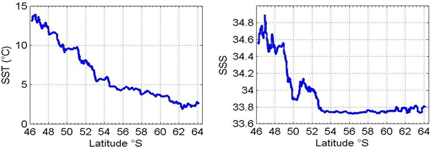
Consequently, here, to determine the number of samples to be collected for AT and CT measurements in the Antarctic and SubAntarctic surface waters, it is essential to fully understand the SST and SSS properties as well as their variability’s. For instance, recently, based upon detailed previous studies [1, 2], Gugliemi V, et al. [3] further showed that over the transect Hobart - Dumont D’Urville the SSS variability is usually much higher than that of SST, especially in the SubAntarctic area. Consequently, SST and SSS properties should ideally be best sampled separately (not simultaneously), with less SST measurements than SSS ones.

Here, using these same underway 2010 SSS and SST data sets with the knowledge of both AT and T as functions of SSS and SST, we will show how to design appropriate sampling patterns for AT and CT according to the accuracies of the different properties to be studied. We will then compare these results with the measured properties.

Materials and Methods

Data Sets

Here, as example, we use the archived (February 19-23, 2010) data set of sea-surface (at around 5m) SSS and SST [3]. These data are part of the SURVOSTRAL program [4]. They were measured when the supply ship “l’Astrolabe” was sailing from Hobart, Tasmania (43°S 147°E) to the French Antarctic base Dumont D’Urville (66°S, 140°E). These thermosalinograph (TSG) data recorded every minute are freely available [5, 6].

As a reminder SSS was measured with an accuracy of ± 0.005 [1]. According to the manufacturer SST was measured with an accuracy of ± 0.001°C.

Figure 1 shows the result of the February 2010, 5978 measurements of these two properties (SST, SSS) along the cruise track from Hobart (Tasmania) to Dumont D’Urville (Antarctica) within the latitudinal interval [46.2°S - 64.1°S], corresponding to the SubAntarctic and Antarctic regions.

Figure 1: SST(°C) and SSS measured every minute as a function of latitude between 46.2°S and 64.1°S.

Method

In order to determine appropriate sampling patterns for underway surface ocean measurements of AT and CT, here we will need to combine two sets of equations; ones from Brandon M, et al. [7], which provide the relationships of AT as a function of SSS and SST, and of CT also as a function of SSS, SST, and the atmospheric CO2 fugacity (fCO2 atm), and others from Davis D, et al. [8], that provide a way to determine the position of the samples to be collected. Thus, below we remind briefly the main equations of Brandon M, et al. [7], as well as those of Davis D, et al. [8]. Then in the following section we provide a concrete application of these equations to determine appropriate sampling patterns for the CO2/carbonate properties.

Equations from Brandon M, et al.

Within this ocean area, using data from the years 2005 through 2019, the authors Brandon M, et al. [7] showed that as a mean over these years, total alkalinity ( ) mean T A and total CO2 ( ) mean T C concentrations, can be quantified with simple multi-linear functions of sea-surface temperature (SST) and salinity (SSS), as follows:

mean mean mean mean T A = a + b *SSS + c *SST (1)

with $a_{\text{mean}} = 762.69; b_{\text{mean}} = 45.28; c_{\text{mean}} = -2.15$ (for both the SubAntarctic and Antarctic regions; $[46.2^\circ; 64.1^\circ\text{S}]$) with an $A_T$ RMSE of $6.8 \mu\text{mol.kg}^{-1}$.

And
$$C_T^{\text{mean}} = a_{\text{mean}} + b_{\text{mean}} \cdot SSS + c_{\text{mean}} \cdot SST + d_{\text{mean}} \cdot \left( fCO_2^{\text{atm}} - 280 \right)$$ (2)

With $a_{\text{mean}} = 1431.45; b_{\text{mean}} = 20.68; c_{\text{mean}} = -10.45; d_{\text{mean}} = 0.56$ for the SubAntarctic region $[46.2^\circ\text{S}; 53.5^\circ\text{S}]$ with a $C_T$ RMSE of $8.9 \mu\text{mol.kg}^{-1}$,

With $a_{\text{mean}} = -269.74; b_{\text{mean}} = 70.42; c_{\text{mean}} = -6.27; d_{\text{mean}} = 0.51$ for the Antarctic region $[53.5^\circ\text{S}; 64.1^\circ\text{S}]$ with a $C_T$ RMSE of $8.5 \mu\text{mol.kg}^{-1}$.

Equations from Davis D, et al.

Based upon the fact that a maximum error function can be determined from both the spacing and variability functions of a signal, one has to calculate the variability function and adjust the spacing function to minimize the maximum error function.

Variability Function

By definition, the signal variability $(\text{VarY(X)})$, of a signal $Y$ as a function of $X$, is similar to the second derivative of the signal and can be calculated as:

$$\text{VarY(X)} = 2 \cdot \left( [\Delta^+ Y / \Delta^- X] / (\Delta^+ X + \Delta^- X) \right)$$ (3)

with $\Delta^+ Y = Y_{i+1} - Y_i; \Delta^- Y = Y_i - Y_{i+1}; \Delta^+ X = X_{i+1} - X_i; \Delta^- X = X_i - X_{i+1}$; for $i = 2, \dots, N-1$.

Where the first “i” starts at the second measured point, up to the one before last.

Maximum Error Functions

The maximum error of interpolation of a regular sampling pattern of $N$ samples points in an interval $[XsI, XeI]$ is given by:

$$\text{MaxErrEven}(N, \text{MaxBndY(X)}, XsI, XeI) = \left( \frac{\text{MaxBndY(X)}}{8} \right) \cdot \left( \frac{XeI - XsI}{(N-1)} \right)^2$$ (4)

Where $\text{MaxBndY(X)}$ represents the maximum of the bound $(\text{BndY(X)})$ of the variability function.

The maximum error of interpolation of a semi-balanced error sampling pattern of $N$ samples points in an interval $[XsI, XeI]$ is given by:

$$\text{MaxErrBal}(N, XsI, XeI) = \left( 1 / \left[ 8(N-1)^2 \right] \right) \cdot \left( \int_{XeI}^{\text{XeI}} \sqrt{BndY(X)} \text{dX} \right)^2$$ (5)

Sample Size

Reversely, using these above Equations (2&3), it is possible to determine the minimum number of samples (sample size) needed to reach an aimed maximum interpolation error $(\text{MaxErrY})$ within a given interval $[XsI, XeI]$.

Where there is a constant bound $(\text{CstBnd})$ of the signal variability function, the number of samples can be calculated from Equation 2 as:

$$\text{SampleSizeEven}(\text{MaxErrY}, \text{CstBnd}, XsI, XeI) = \left( XeI - XsI \right) \cdot \sqrt{\frac{\text{CstBnd}}{8 \cdot \text{MaxErrY}}} + 1$$ (6)

Where the bound of the signal variability function varies, the number of samples can be calculated from Eq.3 as:

$$\text{SampleSizeBal}(\text{MaxErrY}, XsI, XeI) = \int_{XeI}^{\text{XeI}} \sqrt{BndY(X)} \text{dX} + \sqrt{8 \cdot \text{MaxErrY}} + 1$$ (7)

Sample Locations

Within an interval where the bound of the signal variability is constant, the samples will be evenly distributed along the $x$ axis. And within an interval where the bound of the signal variability varies, the samples will be distributed according to the following “Distribute” function:

$$\text{Distribute}(M, A(x)) = \left\{ x_i \mid i = 0, \dots, M-1, x_0 = a \leq x_i \leq b \right\}$$ (8)

Such that $A(x_{i+1}) - A(x_i) = (A(b) - A(a)) / (M-1)$, with $i = 0, \dots, M-1$.

Where $M$ represents the number of points to be distributed within the interval $[a, b]$,

and $A(x) = \int_a^x \sqrt{BndY(t)} \text{d}t$ in this interval $[a, b]$.

Results and Discussion

In order to determine the variability of the $A_T$ and $C_T$ over the latitudes 46.2°S through 64.1°S, the first step is to calculate $A_T$ and $C_T$ mean from equations 1 and 2, respectively.

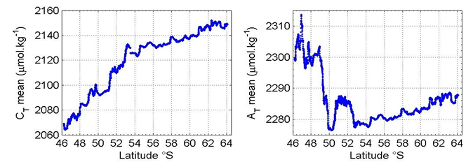
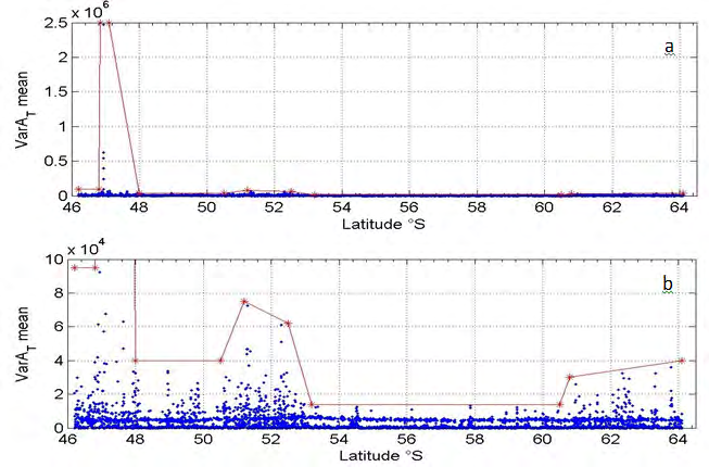
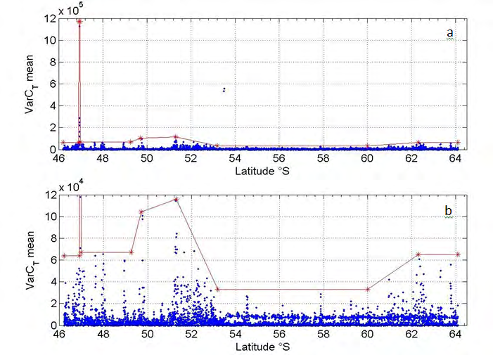
Figure 2: Calculated AT mean (μmol.kg-1) and CT mean(μmol.kg-1) from equations 1 and 2, respectively, as a function of latitude between 46.2°S and 64.1°S (from the SubAntarctic to the Antarctic areas) These results (Figure 2) are then used to compute their variability (eq. 3; Figures 3 & 4) and to determine their variability bounds (Figures 3 & 4).

Figure 3: Variability and variability bounds for AT mean as a function of latitude South, a) full AT variability scale, b) zoom on the AT variability scale.

Figure 4: Variability and variability bounds for CT mean as a function of latitude South, a) full CT variability scale, b) zoom on the CT variability scale.

Since AT in surface seawater is mainly related to salinity, its variability closely follows that of salinity. The variability of CT also follows that of SSS but is significantly mitigated by that of SST.

Thus, the variability bounds are:

BndAT mean(L) = {[46.2, 95000], [46.8, 95000], [46.85, 2500000], [47.1, 2500000], [48.0, 40000], [50.5, 40000], [51.2,75000], [52.5, 62000], [53.2, 14000], [60.5, 14000], [60.8, 30000], [64.1, 40000]}, and BndCT mean(L) = {[46.2, 64000], [46.9, 64000], [46.93, 1170000], [46.96, 1170000], [46.98, 67000], [49.25, 67000], [49.7,104000], [51.3, 116000], [53.2, 33000], [60.0, 33000], [62.3, 65000], [64.1, 65000]}.

As expected, the variability bounds of AT and CT are significantly different. However, in very particular cases they may be similar. Yet, the shapes of these bounds are relatively similar, with a minimum (for both AT and CT) in the latitudinal area [53.2°S - 60.0°S], in the Antarctic zone [9, 10].

Determination of the Aimed Maximum Interpolation Error

Knowing that the accuracy of the AT measurements at sea is 3.5μmol.kg-1, a reasonable maximum interpolated error could be 3.3μmol.kg-1, such that the maximum total error over the whole transect would be 6.8μmol.kg-1, similar to the RMSE of AT mean.

Similarly, knowing that the accuracy of the CT measurements at sea is 2.7μmol.kg-1, a maximum interpolated error could be up to 5.8μmol.kg-1, such that the maximum total error over the whole transect would be 8.5μmol.kg-1, similar to the RMSE of CT mean.

Of course, the choice of the aimed maximum interpolated error could be different according to the given objectives of the scientific studies. For instance, local process studies in ocean acidification [11, 12, 13, 14] would require much more smaller errors than global modeling studies [15, 16, 17, 18].

Determination of the Minimum Sample Size

Within the latitudinal interval [46.2°S; 64.1°S], the minimum sample size for AT measurements, determined using eq.7 for a maximum interpolation error of 3.3μmol.kg-1, is 831. Table 1 summarizes the results assuming different aimed interpolation errors from 1μmol.kg-1 to 4μmol.kg-1.

Latitudinal interval	N SSS & SST measured	N for an Aimed AT Maximum Interpolation Error (μmol.kg-1)
		1	1.5	2	2.5	3	3.3	3.4	4
42.2°S -64.1°S	5978	1508	1232	1067	954	871	831	818	755

Table 1: Number of samples required to reach an aimed AT mean maximum interpolation error.

These results indicate that according to the aimed AT maximum interpolation error, the number of samples for AT measurements can be between 4 and 7 times less than that of the SSS and SST measurements. Yet, this represents a lot of samples, more than 4.5 times the number of AT samples measured (185) during the 2010 cruise.

Within the latitudinal interval [46.2°S; 64.1°S], the minimum sample size for CT measurements, determined using eq.7 for a maximum interpolastion error of 5.8μmol.kg-1, is 619. Table 2 summarizes the results assuming different aimed interpolation errors from 2.5μmol.kg-1 to 6μmol.kg-1.

Latitudinal Interval	N SSS & SST Measured	N for an Aimed CT Maximum Interpolation Error (μmol.kg-1)
		2.5	3	3.5	4	5	5.5	5.8	6
42.2°S - 64.1°S	5978	942	860	796	745	667	636	619	609

Table 2: Number of samples required to reach an aimed CT mean maximum interpolation error. These results show that for an identic

Table 2: Number of samples required to reach an aimed CT mean maximum interpolation error. These results show that for an identical given aimed maximum interpolation error for both AT and CT properties, the number of sample collected should be slightly different. For example, for an aimed maximum error of 3μmol.kg-1, 871 and 860 samples should be collected for AT and CT, respectively. Yet, such numbers of samples are still very high.

Determination of the Sample Positions

Since often a single sample (or duplicate samples at the same location) will be collected for AT and CT measurements, the computation of the sample position should be performed for the property which requires the higher number of samples. Thus, this later property will be correctly sampled to reach its aimed interpolation error, while the other property will be over sampled and will have an interpolation error even smaller than its aimed interpolation error.

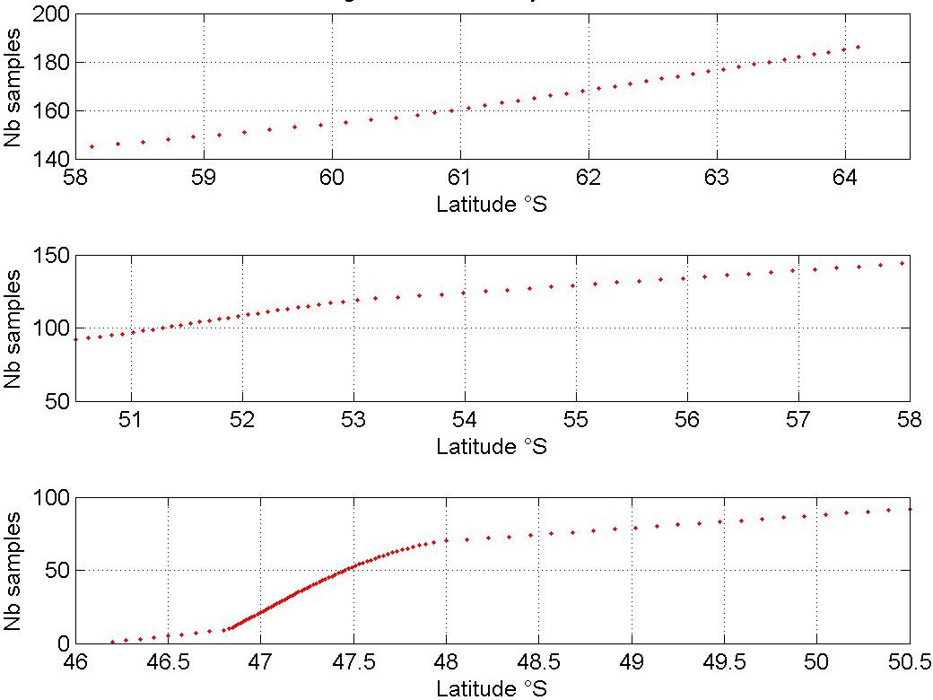
Here, in this example, the higher number of samples to reach the aimed accuracy of AT and CT, is that of AT. Hence, we will use the bound BndAT mean(L) to perform the computation of the samples positions. Thus, using equation 8 with ( ) A(x) dL x $$ ) = \int_ {a} ^ {x} \sqrt {B n d A T m e a n (L)} \mathrm {d L}, $$ the sample positions for the AT and CT measurements are shown in Figure 5.

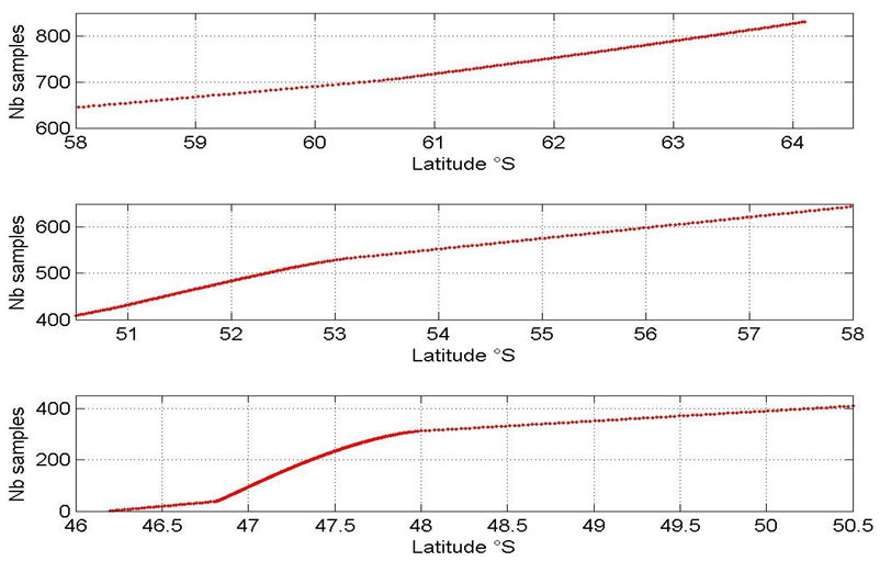
Figure 5: Latitudinal position of the 831 samples needed to reach the aimed maximum error of 3.3μmol.kg-1 for AT interpolation.

Figure 6: Number of samples required for AT measurements within each degree of latitude.

This sampling pattern distribution reflects the amplitudes of the variability bound. Since the largest variability bound is observed within the latitudinal interval [46.8°S; 48°S], the smallest sample spacing is within this interval.

a BndCTmean L = ∫ . The result is shown in Figure 7.

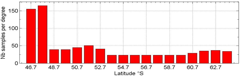
Given the above sample distribution, the number of samples required for AT measurements within each degree of latitude is shown in Figure 6.

Now, if samples for AT and CT can be collected independently, the sample position can be also calculated using equation 8 with ( ) A(x) dL x

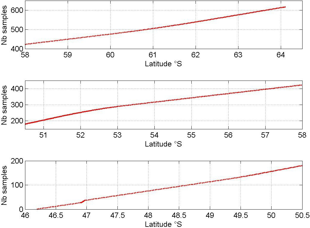
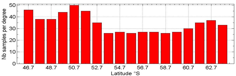
Figure 7: Given the above sample distribution, the number of samples required for AT measurements within each degree of latitude is shown in Figure 6.

Figure 8: Number of samples required for CT measurements within each degree of latitude.

Given the above sample distribution, the number of samples required for CT measurements within each degree of latitude is shown in Figure 8.

Note here the significant difference with the AT sampling pattern especially in the [46.8°S - 48°S] interval in which CT variability is very low compared with that of AT.

This above example assumes there is no constraint on the number of samples to be collected and measured. However, in practice, the number of samples/measurements is often a real constraint. For instance, the number of sample within this latitudinal interval ([46.2°S - 64.1°S]) during the 2010 cruise was limited to 185.

Thus, let’s assume that only 185 samples for AT and CT measurements could be collected over this latitude range [46.2°S; 64.1°S]. Where should they be collected?

In this case, at best, if the samples were appropriately distributed as shown below, the maximum interpolated error for AT will be (from eq. 5) 67μmol.kg-1. Then, using equation 8 also with the same ( ) A(x) dL x $$ 0 = \int_ {a} ^ {x} \sqrt {B n d A T m e a n (L)} $$

, but with M = 185 instead of

831, the sample positions would be as represented in Figure 9.

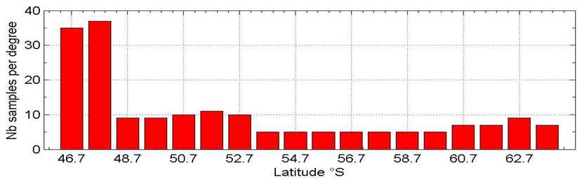
Figure 9: Latitudinal position for the 185 samples for AT measurements.

Figure 10: Number of samples within each degree of latitude required for AT measurements for a limited total of 185 samples.

Given the above sample distribution for the 185 samples for AT measurements, the number of samples within each degree of latitude is shown in Figure 10.

In practice, the samples are quasi-evenly spaced and in such case the maximum interpolation error (without taking into account the high variability around 47°S), which should then be calculated by equation 4, is 118μmol.kg-1.

In other words, we do know relatively accurately AT (or CT) at the measured points but between two measured points the uncertainty can be extremely large, which prevent scientists to reliably (with known uncertainty) analyze the data to improve their studies. This may be a significant issue, in particular for all modeling studies which are required to interpolate the measured data to their specific model grid [15, 16, 17, 18].

For the sake of the discussion and to further show the influence of the accuracy of both the determination of AT and CT as multilinear functions of salinity and temperature, below we used the measured AT and CT data during this 2010 MINERVE cruise [19, 20, 21], to determine the constants for the AT 2010 and CT 2010 relationships.

Thus, if we use only the 2010 data sets, using the same type of equations (1&2) as Brandon M, et al. (2022), the results are:

AT 2010 = a2010 + b2010*SSS + c2010*SST (9)

with a2010 = 529.00; b2010 = 52.38; c2010 = -2.93 for both the SubAntarctic and Antarctic regions [46.2°; 64.1°S] with an AT RMSE of 3,2μmol.kg-1, and CT 2010 = a2010 + b2010*SSS + c2010*SST (10) with a2010 = 2476.45; b2010 = -9.23; c2010 = -7.07 for the SubAntarctic and Antarctic regions [46.2°S; 64.1°S] with a CT RMSE of 4,0 μmol.kg-1.

Note that here, for a single year fCO2 atm is constant, and thus the term d*(fCO2 atm - 280) from eq. 2, is a constant included in the constant a2010. Also, note that only one (instead of two) set of constants is determined for both the SubAntarctic and Antarctic areas (thus avoiding any discontinuity between them).

These results for a single year (2010) show RMSE of both AT 2010 and CT 2010 quasi-identical to the accuracy of the AT and CT measurements on board. These excellent results, not only valid the accuracy of the measurements of the four properties AT, CT, SST and SSS, but also valid the form of the relationships (eq. 1&2), which indicates that AT and CT in surface seawater are simple multi-linear functions of SSS and SST.

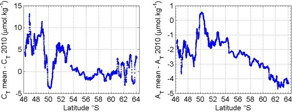
Figure 11: Differences CT mean – CT 2010 and AT mean – AT 2010 as function of latitudes South.

Figure 11 shows the small difference both between AT mean and AT 2010 and between CT mean and CT 2010.

Thus, for AT the differences indicate that compared with AT mean, AT 2010 is shifted by + 2μmol.kg-1 and vary by +/- 2μmol. kg-1 decreasing with Southward latitudes. While for CT the differences (CT mean- CT 2010), remain within +/- 4μmol.kg-1 in the Antarctic region. In the SubAntarctic area CT 2010 is shifted by - 5μmol.kg-1 with larger differences (+/- 7μmol.kg-1) compared with CT mean.

Thus, in order to take full advantage of the good accuracy of both, the measurements and the interpolations, it is essential to judiciously choose the locations of the samples and to accurately define the dependence of AT and CT with SSS and SST. The fulfillment of these conditions will open the route to significant progresses in data analyses.

Conclusions

The first thing about sampling the ocean is to sample it anyway you can to get an idea of the behavior of its variability, and to see if the shape of the variability over the region sampled is consistent. If it is not consistent, then all you can continue to do, is to sample it as much as you can wherever you can.

Once a consistent variability is known, then it is possible to sample more efficiently and more scientifically using semi- balanced error sampling. Semi-balanced error sampling provides samples of the data field that can be used to interpolate the value of the data field at points not sampled with a more uniform accuracy, which has greater scientific value and usefulness than a sample where the interpolation error is unknown or is highly variable.

The chief property of the data variability, or a bound of its absolute value over the region to be sampled, is that its shape determines the shape of a balanced sample pattern. This follows from the Sample Error Theorem. The sample spacing for a balanced error sample is low where the variability is high. Or more simply, the sampling rate is high where the variability is high. That is what balances the error and makes it uniform. This relationship is scale invariant. Multiply the bound by a constant and the shape of the balanced error pattern stays the same.

However, there is also a relationship between the maximum error of a balanced sample pattern and its size (number of samples) that is determined by the magnitude of the variability and its bound, not just its shape. This is one of the precise results of the mathematical analysis. This has great scientific usefulness, since knowing a bound on the magnitude of data variability, a scientist can determine beforehand how many samples have to be taken to achieve a given maximum interpolation error. This assumes of course that the sample pattern is a semi-balanced error pattern.

It should be emphasized that if two properties have the same shape of variability (such as temperature and salinity in our examples), they are good candidates to be measured together even if their magnitudes of variability are very different. But of course, they cannot be efficiently measured together unless their sample sizes are the same or almost the same. But their sample sizes are determined by the requirement for interpolation accuracy (or a maximum bound on sample error), which is determined by the magnitude of their variability. Their requirements for accuracy may be on very different scales, so unless their magnitudes differ in the same way as their required accuracy scales, it will not be possible to efficiently measure them together.

A final principle is the fact that the more you sample a data field accurately using semi-balanced error samples, the more you know about the variability and thus the more you can improve the accuracy of your sampling. Basically, this methodology improves on itself every time it is used, because its improved accuracy enables further improvement. And all of these principles are backed by specific tools of analysis.

One of the most common error in ocean data sampling is that all the different measurements are often taken at the same even rate, but the requirement that their variability shapes and magnitudes be compatible is not even known, and therefore ignored. As a result, the use of such data for interpolation may lead to unknown results.

These simple principles form the basis of a practical scientific approach to sampling all backed by a rigorous mathematical foundation and results.

Acknowledgments

We genuinely thank Alain Poisson for the initiation of the MINERVE program, as well as Elodie Kestenare and Rosemary Morrow for the SURVOSTRAL data and helpful comments. We are grateful to Daniel Davis for helpful discussions, thoughtful suggestions, and providing language help. We thank the Terres Austral et Antactique Françaises (TAAF) and the Institut Paul Emile Victor (IPEV) for logistic support during the 2010 cruise.

Funding

This research did not receive any grant from funding agencies in the public, commercial, or not-for-profit sectors.

References

Morrow R, Kestenare E (2014) Nineteen-year changes in surface salinity in the Southern Ocean south of Australia. Journal of Marine Systems 129: 472-483.
Morrow R, Donguy JR, Chaigneau A, Rintoul S (2004) Cold core anomalies at the SubAntarctic Front, south of Tasmania. Deep-Sea Research part I: Oceanographic Research Papers 51(11): 1417-1440.
Guglielmi V, Touratier F, Goyet C (2022) Mathematical determination of discrete sampling locations minimizing both the number of samples and the maximum interpolation error: application to measurements of surface ocean properties. EarthArxiv, pp: 1-26.
LEGOS, Laboratory of Geophysics and Spatial Oceanography Studies.
Sea Surface Salinity Data Base Web Access.
Alory G, Delcroix T, Techine P, Diverres D, Varillon D, et al. (2015) The French contribution to the voluntary observing ships network of sea surface salinity. Deep Sea Research Part I: Oceanographic Research Papers 105: 1-18.
Brandon M, Goyet C, Touratier F, Lefèvre N, Kestenare E, et al. (2022) Spatio- temporal variability of the CO2 properties and anthropogenic carbon penetration, in the Southern Ocean surface waters. Deep Sea Research Part I: Oceanographic Research Papers 187: 103836.
Davis D, Goyet C (2021) Balanced Error Sampling: With application to ocean biogeochemical sampling. Presses Universitaires de Perpignan, pp: 214.
Orsi AH, Whitworth T, Nowlin WD (1995) On the meridional extent and fronts of the Antarctic Circumpolar Current. Deep Sea Research Part I: Oceanographic Research Papers 42(5): 641-673.
Chaigneau A, Morrow R (2002) Surface temperature and salinity variations between Tasmania and Antarctica, 1993-1999. J Geophys Res 107(c12): SRF 22-1-SRF 22-8.
Krasakopoulou E, Souvermezoglou E, Giannoudi L, Goyet C (2017) Carbonate system parameters and anthropogenic CO2 in the North Aegean Sea during October 2013. Continental Shelf Research 149: 69-81.
Cai WJ, Feely RA, Testa JM, Li M, Evans W, et al. (2021) Natural and Anthropogenic Drivers of Acidification in Larges Estuaries, Annual Review of Marine Science 13: 23-55.
Hurst TP, Copeman LA, Andrade JF, Stowell MA., Al- Samarrie CE, et al. (2021) Expanding evaluation of ocean acidification responses in a marine gadid: elevated CO2 impacts development, but not size of larval walleye pollock. Marine Biology 168(8).
Dickinson G H, Bejerano S, Salvador T, Makdisi C, Patel S, et al. (2021) Ocean acidification alters properties of the exoskeleton in adult Tanner crabs, Chionoecetes bairdi. The Journal of experimental biology 224(3): jeb2328.
Pousse E, Daphne M, Hart D, Hennen D, Cameron PL, et al. (2022) Dynamic Energy Budget modeling of Atlantic surfclam, _Spisula solidissima_, under future ocean acidification and warming. Marine environmental research 177: 105602.
Khatiwala S, Primeau F, Hall T (2009) Reconstruction of the history of anthropogenic CO2 concentrations in the ocean. Nature 462(7271): 346-349.
Sallee JB, Shuckburgh E, Bruneau N, Meijers AJS, Bracegirdle TJ, et al. (2013) Assessment of Southern Ocean water mass circulation and characteristics in CMIP5 models: Historical bias and forcing response. J Geophys Res Ocean118(4): 1830-1844 .
Schlund M, Lauer A, Gentin, P, Sherwood SC, Eyring V (2020) Emergent constraints on equilibrium climate sensitivity in CMIP5: do they hold for CMIP6? Earth Sys Dyn 11: 1233-1258.
French Oceanographic Campaigns, MiNERVE, Series of oceanographic cruises.
Marine Data Portal, Sismer, French research institute for the exploitation of the sea.
Seanoe Sea scientific open data publication.

← Previous Article Long-Term Changes in Winter SST, Wind Stress and Anchovy Fishery in Relation to Climatic Indices along the South-Eastern Black Sea Next Article → New Administrative Territories in Indonesia and its Implications to Fisheries Extension Activities