Cox-Lognormal Model to Assess Longevity in Curraleiro Pé Duro Cattle Breed from the Semiarid Region of Brazil
Cattle of the Curraleiro Pé Duro breed are characterized as very docile and exceptionally rustic animals. They are animals gradually adapted to low quality native pastures, drought conditions, high temperatures and other adverse factors, resulting in the formation of bovine herds adapted and resistant to the unfavorable conditions of the Brazilian hinterland. In this context, the objective of this work was to use the survival analysis methodology with a Cox-lognormal proportional hazards model, to assess the stayability in the herd, considering the failure as the inactivity of the bovine being caused by death or sale, using information from 102 Curraleiro Pé Duro cattle born in the period from 2005 to 2014 in an experimental field of Embrapa Meio-Norte located in São João do Piauí. The Cox-lognormal proportional hazards model considered, among the analyzed covariates, the season of birth, sex and weight at 365 days as significant. There was a predominance of birth in the dry season (July to December). It was observed that the cattle that longer remained in the herd were born in the dry season, were male and weighed less than 95 kg at 365 days, justified by the absence of parasites, availability of pasture for the mother during the pregnancy period, carcass evaluation, sale, slaughter and reproduction. The Cox-lognormal proportional hazards model proved to be adequate in the adjustment of the statistical model to estimate the stayability in the herd, with censorship related to the inactivity of the Curraleiro Pé Duro breed.
Introduction
The Curraleiro Pé Duro breed, recognized by the Ministério da Agricultura, Pecuária e Abastecimento (Ministry of Agriculture, Livestock and Supply) in 2012, is the first breed selected in Brazil. This local breed, also known as native, naturalized or creole, is a historical and cultural heritage in Piauí and helped the country’s economic development as a means of transport, a source of protein, and a trade in jerked beef and leather. The researchers’ attention to this breed came from the observation of how these cattle gradually adapted to low-quality native pastures, dry conditions, high temperatures, among other adverse factors to cattle breeding in Brazil. These adaptation mechanisms have occurred over the centuries, resulting in the formation of bovine herds adapted and resistant to the unfavorable conditions of the Brazilian hinterland. The animals’ ability to adapt to extreme weather conditions (high temperatures, drought) in a natural environment favored the minimization of losses in productive and reproductive performances, helping in disease resistance, consequently reducing mortality and increasing longevity when exposed to conditions of stress [1].
The survival analysis, in turn, is considered the most appropriate statistical methodology to deal with time data to the occurrence of an event of interest (time of failure), in the presence of censorship which is its main feature. In the animal production area, the survival characteristics are: longevity (age of the animal at disposal) [2]; productive life span (interval from first birth to disposal); number of lactations during life and ability to remain in the herd or staybility. The survival analysis methodology has already been used by some authors in the study of dairy cattle longevity. Bonetti, et al. [3] estimated genetic parameters in a genetic evaluation for the longevity of Italian Brown-Swiss bulls using the Weibull proportional hazards model. The authors considered the method satisfactory for the use and inclusion of bulls in genetic improvement programs. Caetano, et al. [4] proposed the cow’s age at last calving as a measure to assess the cow’s ability to remain in the herd. The authors concluded that the variable is relevant to assess the ability of cows to remain in the herd and that the survival analysis model was the one that estimated the highest proportion of genetic variability for the trait studied. Other authors who used this methodology were: Giolo [5], Van Melis, et al. [6] and Kern, et al. [7].
A special feature associated with survival data is the possibility that, for some individuals, the complete time until the occurrence of the event of interest is not observed due to many causes. For example, an individual can remain in follow-up until the end of the study period without having experienced the event of interest. Failure to consider these individuals with incomplete information about their lifetimes can lead to biased or less efficient inferences. Therefore, one can see the importance of introducing a variable in the analysis that indicates whether the survival time was observed [8]. This variable is defined in the literature as a censorship indicator variable. Censorship is said to be type I when it occurs due to the end of the study after a predetermined period of time; type II, when it occurs due to the end of the study after a previously fixed number of failures; or it can be random, being the most common in practical situations. The previously mentioned censors are known as right censorship, as the failure always occurs to the right of the recorded time. There are also other censorship mechanisms, such as left censorship, in which the recorded time is greater than the failure time, and interval censorship, in which the exact failure time is not known, where the only information available is that the failure time occurred within a certain time interval. In this research, however, only the right censorship mechanism, which will be called “censorship”, will be adopted. The main objective of this study was to evaluate the survival time or permanence in the herd of the Curraleiro Pé Duro breed, related to exit from the herd due to death or sale, using the methodology of parametric Cox models with lognormal basis risk function.
Materials and Methods
Description of the Data
The data for this study were provided by the Curraleiro Pé Duro (CPD) bovine conservation center belonging to Embrapa Meio-Norte, in Teresina-Piauí-Brazil, with an experimental field located on the Otávio Domingues farm, in São João do Piauí (between 8° 26’ and 8° 54’ South latitude and between 42° 19’ and 42° 45’ West longitude), in the semiarid region of Piauí belonging to an in situ conservation herd. Cattle are bred extensively with the supply of only salt, minerals and water, which justifies their low weight compared to CPD cattle raised in other regions and other breeds. Also, due to the lack of food supplementation, there is an increased incidence of environmental effects, with the presence of many toxic plants, ticks, babesia, and worms, among others. 102 cattle (58 males and 44 females) of the CPD breed were evaluated from birth to 550 days. Animal data were collected from 2005 to 2014. To model the survival time (in months), after the beginning of the reproductive life of the cattle until the occurrence of failure (inactivity caused by death or sale), in relation to the cattle remaining active (alive), time was considered as the response variable, and the calf’s date of birth was the beginning of the study. The variable T (time) was obtained from the difference between the date of birth and the date of disposal. The date of the last disposal in the herd was considered as the final observation period for animals that had not been disposed yet (08/19/2016). Failure was defined as cattle inactivity (death or sale), while censorship was defined for cattle that remained alive in the herd. The type of censorship used was the right one. For each animal observed, it was registered a corresponding indicator of censorship, called status (δ=1 if it failed and δ=0 if censored) indicating whether the animal is active or inactive in the herd. The variable season was considered to be rainy in the period from January to June and dry in the period from July to December. The covariates considered as possible risk factors in the stayability of CPD cattle in the herd were: SB: season of birth (0 - rainy, 1 - dry), S: sex (0 - male, 1 - female), BW: birth weight (0 - < 20kg,
1 - ≥ 20kg), WW: weaning weight (0 - < 66kg, 1 - ≥ 66kg), W365: weight at 365 days (0 - < 95kg, 1 - ≥ 95kg), W550: weight at 550 days (0 – < 131kg, 1 – ≥ 131kg) categorized according to the average weight in each phase (12).
Statistical Analysis
The Cox regression model was proposed by Cox in 1972 and it allows the analysis of data from lifetime studies in which the answer is the time until the occurrence of an event of interest, adjusting for covariates [2]. The model proposed by Cox directly models the risk function and has as its basic principle to estimate the effect of covariates, the proportionality of the risks throughout the observation period.
The proportional risk model is given by:
$$ h \left(t | \mathrm {x}\right) = h _ {0} (t) \exp \left(\boldsymbol {\beta} ^ {\prime} \mathrm {x}\right) $$ (1) where h0(t) is the base risk function, that is, the risk of an animal with covariates equal to zero; β = (β1,...,βk) is the k-dimensional vector of unknown regression coefficients and x = (x1,...,xk) is the k-dimensional vector of covariates for the i-th observation. Model (1) is composed of the product of two components: ( ) ' exp β x which measures the effect of covariates and h0(t) which can be parametric or not. In the semiparametric case the component h0(t) is considered to be a non-negative function of time; when parametric, it can assume distributions such as Gompertz, lognormal, gamma and others. This model is also called the proportional risk model, since the failure rate ratio of two different individuals is constant over time. That is, the ratio of the failure rate functions for individuals i and j given by:
$$ \frac {h \left(t \mid x _ {i}\right)}{h \left(t \mid x _ {j}\right)} = \frac {h _ {0} (t) \exp \left\{\boldsymbol {\beta} ^ {\prime} x _ {i} \right\}}{h _ {0} (t) \exp \left\{\boldsymbol {\beta} ^ {\prime} x _ {j} \right\}} = \exp \left\{\boldsymbol {\beta} ^ {\prime} \left(x _ {i} - x _ {j}\right) \right\} $$ doesn’t depend on time. For example, if an individual at baseline has a death risk equal to twice as much as the risk of a second individual, then this hazard ratio will be the same for the entire follow-up period [2].
The interpretation of the coefficients in a Cox regression model is performed using the exp (βi) quantities, called the risk or failure rate ratio (RTF). A value of βi greater than zero, or equivalent to a hazard ratio greater than one, indicates that, as the value of i-th covariates, the risk of failure increases and, therefore, the time of survival decreases. Thus, if RTF= 1 it is said ineffective; if RTF < 1 there was a reduction in risk and if RTF > 1 there was an increase in risk. In the Cox model, the survival function is defined by:
( ) ( ) { } { } ( )
$$ \left| \boldsymbol {x} _ {i}\right) = \exp \left\{- \int_ {0} ^ {t _ {i}} h _ {0} (u) \exp \left\{\beta^ {\prime} \mathrm {x} \right\} d u \right\} = \left[ S _ {0} \left(t _ {i}\right) \right] ^ {\exp \left\{\beta^ {\prime} \mathrm {x} \right\}} $$ it exp x x ix i i S t exp h u exp du S t where S0(ti) is the basic survival function, that is, the survival function of an animal with all covariates equal to zero. The basis cumulative risk function, H0(t), is given by 𝐻0 (𝑡) = − 𝑙𝑜𝑔(𝑆0(𝑡)).
In this study, the parametric approach for the Cox model is considered, where the lifetimes of cattle at risk follow lognormal distribution. Table 1 shows the probability density functions f(t), risk h0(t) and survival S0(t) for the lognormal, log-logistical and Gompertz distributions, which serve as a comparison for the proposed Cox-lognormal.
| Distribution | f(t) | h (t) 0 | S (t) 0 |
|---|---|---|---|
| Log Normal | 1 1 log(t )−µ2 exp− 2π tθ 2 σ | 1 1 log(t )−µ2 exp− 2π tθ 2 σ −log(t )+µ Φ σ | −log(t )+µ Φ σ |
| Log-Logistic | γ−2 γ t tγ−11+ λy λ | γ−1 t γ λ t γ λ1+ λ | 1 γ t 1+ λ |
| Gompertz | λ λexp(γt)exp− (eγt −1) γ | λexp(γt) |
Table 1: Density functions f(t), survival S0(t) and risk h0(t) of the log Normal, Log-Logistic and Gompertz distributions.
Thus, substituting the basis risk functions h0(t) and basis survival S0(t), from lognormal, respectively in (1) and (2), we have the Cox-lognormal proportional hazards model whose risk function is thus defined:
$$ ) = \frac {\frac {1}{\sqrt {2 \pi t \theta}} \exp \left[ - \frac {1}{2} \left(\frac {\log (t) - \mu}{\sigma}\right) ^ {2} \right]}{\Phi \left(\frac {- \log (t) + \mu}{\sigma}\right)} e $$
2
1 1 log( ) exp 2 2 ( / ) exp( ' ) t
t t h µ $$ \frac {\sqrt {2 \pi t \theta} \exp \left[ - \frac {1}{2} \left(\frac {\log (t) - \mu}{\sigma}\right) \right]}{\Phi \left(\frac {- \log (t) + \mu}{\sigma}\right)} \exp \left(\beta^ {\prime} x\right) $$ t x x µ σ ( ) log( ) and the survival function is rewritten by exp{ ' } log( ) ( / ) x $$ ) = \left[ \Phi \left(\frac {- \log (t) + \mu}{\sigma}\right) \right] ^ {\exp \left\{\beta^ {\prime} x \right]} $$ i i t S t x For inference of parameters, the maximum likelihood method was used. Assuming that the data are independent and identically distributed, the likelihood function, with censored data, according to Lawless [9] is defined by:
$$ L (\theta) = \Pi_ {i = 1} ^ {n} \left[ h \left(t _ {i} / x _ {i}\right) \right] ^ {\delta_ {i}} S \left(t _ {i} / x _ {i}\right) $$ where δi is the censorship indicator. Thus, the data set G = (n,t,δ,X) is formed by the observed failure times 𝒕 = (𝑡1, . . . , 𝑡𝑛), censored failure times 𝜹 = (𝛿1, . . . , 𝛿𝑛)′ and X the n × k matrix containing the covariates, respectively. Replacing (3) and (4) in (5), we have The maximum likelihood estimates are obtained by numerically maximizing the log-likelihood function (log[L(θ)]). The optim package of the R software and the “BFGS” method were used for maximization. The construction of confidence intervals concerns the asymptotic distribution of the maximum likelihood estimator ˆθ . For large samples, under certain regularity conditions, the vector distribution ˆθ =(( ˆθ 1 ),…, ( ˆθ k ),)´ is multivariate normal of mean θ and variance-covariance matrix Var( ˆθ ), that is, ˆ ˆ
( ,var( ))
$$ \hat {\theta} \approx N _ {k} (\theta , \operatorname {v a r} (\hat {\theta})) $$ For the construction of confidence intervals an estimate for the standard error of ˆθ is necessary, that is, for [Var( ˆθ )]1/2. In the special case where θ is a scalar, an approximate interval of (1 − α) 100% confidence for θ is given by For a model with a vector ( ) 1, , p θ θ θ = … ' of parameters, there is often an interest in testing hypotheses related to this vector or a subset of it. Three tests are generally used for this purpose: the Wald, the Likelihood Ratio (TRV) and the Score [2]. Model selection criteria such as the Akaike information criterion (AIC) proposed by Akaike [10] and the Bayesian information criterion (BIC), proposed by Schwarz, et al. [11], are often used to select models in different areas. The best models are considered those with lower AIC and BIC values. For the adequacy of the model, several methods are available in the literature and they are essentially based on Cox-Snell residues, which help to examine the global adjustment of the model, Schoenfeld’s, which has a time-dependent coefficient, the one of martingale, which is given by the difference between the observed number of events for an individual and the expected one, given the adjusted model, and the one of deviance, which facilitate the detection of atypical points (outliers).
Results
In this study, the herd consists of 102 cattle (58 males and 44 females) of the CPD breed born between 2005 and 2014. When considering the survival of these animals in the herd, it was found that 28% remained alive until the final period of observation, that is, 8/19/2016, these being considered as censorship and 72% failed, that is, died or were sold. In that study, there was a predominance of birth in the dry season that encompasses the months from July to December, corresponding to 65.7%. Animals that failed (death or sale) occurred more frequently than animals that remained alive, that is, they were censored. Regarding lifespan, Figure 1 represents the empirical survival function estimated by the non-parametric Kaplan-Meier estimator.
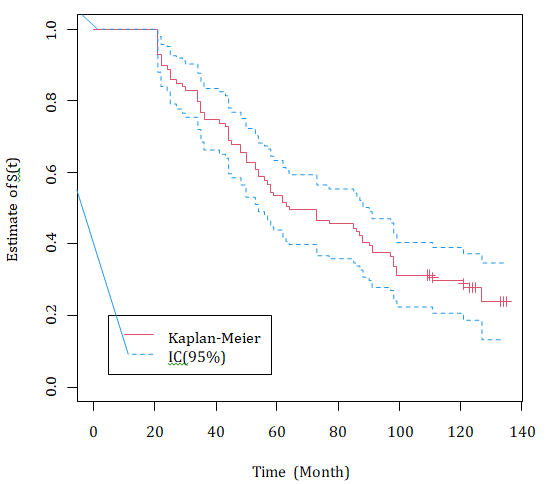
It is possible to verify that 50% of the cattle had a lifespan greater than 63.5 months. In order to analyze whether there is a difference between the survival of the categories for the possible covariates, the referred stratified survival curves are given in Figure 2.
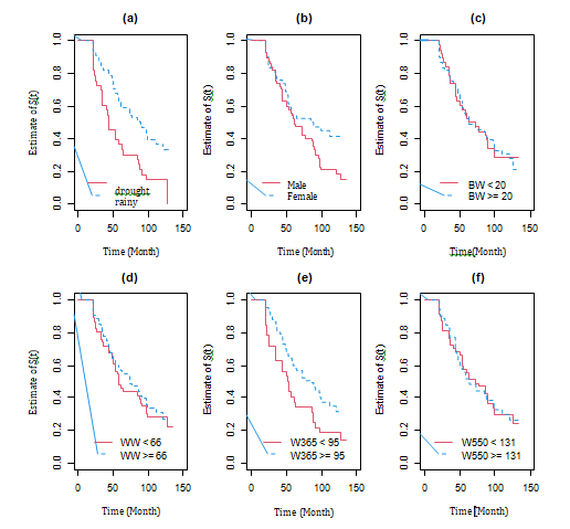
The empirical analysis suggests that there is a difference between the survival of the categories for the SB and W365 covariates and a slight difference in the S covariate. From the Log-rank test, adopting a significance level less than or equal to 10%, significance was observed for SB (p−value = 0.0004), S (p−value= 0.04) , and the W365 (p−value = 0.008). For the other covariates, there was no significant effect between the categories of covariates, that is, for BW (p−value = 0.7), WW (p−value = 0.7) and W550 (p−value = 0.9) for estimating survival probabilities.
In the present work, the lognormal distribution was used and, for comparison purposes, the Gompertz nd log-logistic distributions. The construction of the Cox-lognormal model to analyze the influence of covariates on the cattle stayability in the herd from birth started from a model without covariates and then evaluated the inclusion of covariates and interactions, using the Likelihood Ratio Test (TRV) criterion. Variables that remained significant, considering α = 10%, entered the model. They are: SB, S and W365.
| EMV | SE | CI (95%) | p-value | RTF | |
|---|---|---|---|---|---|
| μ | 3.959 | 0.133 | [3.69; 4.21] | < 2e-16 | - |
| σ | 0.5804 | 0.063 | [0.45; 0.70] | < 2e-16 | - |
| β1 (SB) | -1.269 | 0.272 | [-1.80;-0.73] | 2.96E-06 | 0.281 |
| β2(S) | 1.5811 | 0.406 | [0.78; 2.37] | 9.67E-05 | 4.86 |
| β3 (W365) | 0.7476 | 0.336 | [0.08; 1.40] | 0.026 | 2.112 |
| β4 (S* W365) | -3.065 | 0.564 | [-4.17;-1.95] | 5.50E-08 | 0.047 |
Table 2: Estimates of maximum likelihood (EMV), standard error (SE), confidence interval (CI 95%), p-value and failure rate ratio
According to Table 2, the failure rate in the dry birth season was 0.2811 times, indicating that there is a decrease in the risk of cattle failing (death or sale), among those that manage to stay alive, demonstrating a greater longevity of the beef cattle in the herd. For variable S, the failure rate for females was 4.8602 times the failure rate for males, that is, female calves are 4.8602 times more likely to fail (death or sale) than male calves. For the interaction of variable S with W365, a failure rate of 0.0466 was observed, indicating a decrease in the risk of cattle failing, that is, dying or exiting for sale.
The risk functions in (3) and survival in (4) for the final model are described, respectively, by:
$$ ) = \frac {\frac {1}{\sqrt {2 \pi} 0 . 5 8 0 4 t} \exp \left[ - \frac {1}{2} \left(\frac {\log (t) - 3 . 9 5 9 0}{0 . 8 0 4}\right) ^ {2} \right]}{\Phi \left(\frac {- \log (t) + 3 . 9 5 9 0}{0 . 5 8 0 4}\right)} $$
2 1 1 log( ) 3.9590 exp 2 0.804 2 0.5804 ˆ ˆ ( / ) ( ) log( ) 3.9590 0.5804
t t h t x g x t π β i
and ˆ ( ' ) log( ) 3.9590 ˆ( / ) 0.5804
i g x $$ = \left[ \Phi \left(\frac {- \log (t) + 3 . 9 5 9 0}{0 . 5 8 0 4}\right) \right] ^ {g (\hat {\beta} ^ {\prime} x)} $$ i i t S t x $$ g \left(\hat {\beta} ^ {\prime} x _ {i}\right) $$ Where = exp(−1.2689 × SB + 1.5811 × S +
0.7476 × W365 − 3.0648 × S ∗ W365).
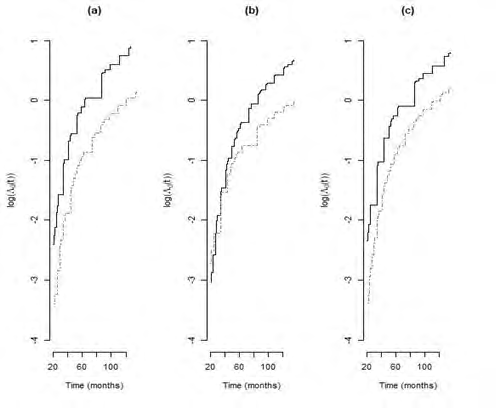
For the model to be suitable for the study, the assumptions of proportionality for the Cox model had to be checked. Through the descriptive graphic method, which involves the logarithm of the accumulated failure function versus time for the covariates: SB (a), S (b) and W365 (c), it was observed that the covariates SB and W365 perfectly meet the proportionality, however, for sex, although they are not perfectly parallel in the beginning, there is, in descriptive terms, no violation of the assumption of proportional failure rates (Figure 3).
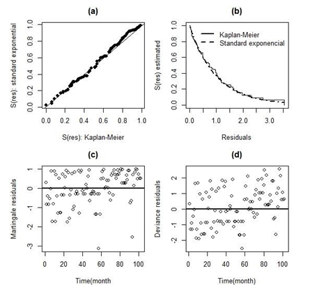
To check the quality of the adjusted model and possible outliers, graphs of Cox-Snell residues, martingale residues and deviance residues are built (Figure 4).
The residuals of Cox, et al [14] help to examine the global adjustment of the parametric model. The closer the survival curves obtained by Kaplan-Meier and the standard exponential model, the better the adjustment of the models to the data is considered. Thus, the survival curves for Cox- Parameters log normal log logistic Gompertz µ 3.959 0.1329 - - - - σ 0.5804 0.0627 - - - - α - - 45.7043 1.3193 - - γ - - 3.1859 0.3661 0.0148 0.0036 λ - - - - 0.0092 0.0025 Snell residuals are presented by graphs (a) and (b) indicating a good quality of the global adjustment of the Cox-lognormal parametric model. Graphs of Martingale residuals (c) and Deviance residuals (d) suggested the absence of outliers.
For comparative purposes, a study was carried out for the Cox-lognormal proportional hazards model with the Cox- log logistic and Cox-Gompertz models.
Estimates Standard Error Estimates Standard Error Estimates Standard Error
- β1(SB)
- -1.2689
- 0.2715
- -1.7489
- 0.4425
- -1.4178
- 0.4014 β2(S)
- 1.5811
- 0.4055
- 1.6139
- 0.3962
- 1.2463
- 0.3787 β3(W365)
- 0.7476
- 0.3358
- 1.022
- 0.4593
- 0.7954
- 0.4263 β4(S*W365)
- -3.0648
- 0.564
- -2.8626
- 0.5006
- -2.5037
- 0.4872
- Log-Veross
- -372.9956
- -374.4386
- -388.4093
- AIC
- 757.9912
- 760.8772
- 788.8186
- BIC
- 773.741
- 776.6271
- 804.5685
Table 3: Estimates for the proportional hazards model parameters of Cox-lognormal, Cox-log logistic and
Table 3 shows the maximum likelihood estimates for the parameters of the proposed models. The selection of models using the Akaike criteria (AIC) showed that, despite the values for lognormal and log-logistic being very close when compared to Gompertz, the Cox-lognormal model was the most suitable, as it had the lowest AIC value, which indicates that this model has a better adjustment quality to the estimated survival times.
Discussion
There are several factors that interfere with the permanence of cattle in the herd. We can highlight birth weight, which is one of the most important factors in the profitability of the cattle herd and has a great influence on survival at weaning [12]. Controlling birth weight is of paramount importance and can be done in two ways: through nutrition and genetics. Birth weight is influenced by race, sex, year (rainfall that affects the availability of pastures, occurrence of diseases, changes in management and genetic progress) and month of birth (dry or wet season, food supply by the mother and the environment ), paternal (size) and maternal (age) effects, in addition to possible interactions between variables. Seasons have a great influence on the birth of calves, and drought is considered a great period for having less diseases for the calves, in addition to the supply of nutrients in the pasture at the time of pregnancy for the mother. Animals that are heavy at birth are usually heavy at weaning due to maternal influence, that is, bovines with a lot of milk have heavier calves, with influence extending up to 1 year. After this period, the animal’s genetics is then observed, when selection is made and adaptability is evaluated. Adaptability, or ability to adapt, can be assessed by the animal’s ability to adjust to average environmental conditions as well as to climatic extremes. Well-adapted animals are characterized by maintenance or minimal reduction in productive performance, high reproductive efficiency, resistance to diseases, longevity and low mortality rate during exposure to stress [1]. In the present study, there was a predominance of 65.7% of calves born in the dry season, indicating that more than half of the calves were born in a favorable period for their development. Furthermore, 50% of the cattle had a lifespan greater than 63.5 months. The perspective addressed in this research was supported by the longevity of cattle and the exit caused by death or sale. Through Figure 2, it was empirically observed differences between the categories of covariates SB, S and W365. The verification of the statistical evidence of this difference was performed using the log-rank test at a significance level less than or equal to 10% under the hypothesis of equality of the survival curves, where the covariates SB, S and W365 remained significant, that is, there is a difference between the dry and rainy season, between males and females and the weight at 365 is less than 95 kg and equal to or greater than 95 kg. The methodology used in this study proved to be promising and had its proportionality assumptions met (Figure 3), a criterion required for the use of Cox’s proportional hazard models and with interesting results in the study to assess the permanence of animals in the herd. The Cox model was used with lognormal basis risk, where significance (p-value < 10%) was found for the covariates: SB, S and W365 and the interaction of S with W365, as shown in Table 2. Still according to Table 2, it was observed through the reason of the failure rate, that for the covariate SB there was a decrease in the failure rate (death or sale) for cattle born in the dry season, which can be explained by having fewer diseases for the calves, besides supply of nutrients in the pasture at the time of pregnancy for the mother, showing a greater longevity for the cattle. For variable S, a higher failure rate was found for females than that for males, which can be explained by the fact that in the carcass evaluation only males go to slaughter. Also, as females give birth annually, in the absence of supplementation, they take it from the bones to put in the milk during breastfeeding, making the cow leaner and more subject to mortality. For variable W365, a higher failure rate was found for cattle weighing 95 kg or more, as heavier cattle leave the herd for sale, slaughter or reproduction. For comparative purposes, the study was carried out for the Cox model with basis risk function, given by the log-logistic and Gompertz distributions, which despite having estimates very close to the lognormal, had a higher AIC and BIC, concluding that the model that best adjusts is the Cox-lognormal model as it has a smaller AIC and BIC. The verification of adjustment quality was performed using the Cox-Snell, Martingale and Deviance tests (Figure 4), indicating the adequacy of the model and the absence of outliers. The methods presented in this study, through survival analysis, can contribute to breeding programs in animals of zootechnical interest in relation to their performance. The methodology can be applied to study the longevity of breeders, associated with points of fragility of a genetic or environmental nature, that is, unobservable factors that negatively affect reproductive and productive efficiency as well as to model the time it takes the animal to achieve a certain weight or daily weight gain, predefined, in a production system focused on animals for slaughter or even on the selection of males and/or females with higher performance.
Conclusion
The Cox-lognormal proportional hazards model proved to be adequate in the verification of observed factors that influence the longevity of these animals, considering the exit of the cattle from the herd either by death or sale. Calves born in the dry season tend to live longer. In relation to sex, females live less than males. However, cattle that weigh at 365 days above the average weight (95 kg) tend to live less. It is noteworthy that other factors that are difficult to measure could not be evaluated with the application of the model, and frailty models, which are an extension of Cox’s proportional risk models, are used for this purpose.
Conflict of Interest Declaration
The authors declare there are no competing interests.
Funding
This research did not receive any specific grant from funding agencies in the public, commercial, or not-for-profit sectors.
References
-
Baccari Júnior F (1990) Métodos e técnicas de avaliação da adaptabilidade dos animais às condições tropicais. Simpósio Internacional de Bioclimatologia Animal nos Trópicos: pequenos e grandes ruminantes 1: 9-17.
-
Colosimo EA, Giolo SR (2006) Análise de sobrevivência aplicada. Editora Edgard Blucher.
-
Bonetti, O, Rossoni A, Nicoletti C (2009) Genetic parameters estimation and genetic evaluation for longevity in italian brown swiss bulls. Italian Journal of Animal Science 8(S2): 30-32.
-
Caetano S, Rosa G, Savegnago R, Ramos S, Bezerra L, et al. (2013) Characterization of the variable cow’s age at last calving as a measurement of longevity by using the kaplan–meier estimator and the cox model. Animal 7(4): 540-546.
-
Giolo SR (2003) Variáveis latentes em análise de sobrevivência e curvas de crescimento. PhD thesis, Universidade de São Paulo.
-
Van Melis M, Eler J, Rosa G, Ferraz J, Figueiredo L, et al. (2010) Additive genetic relationships between scrotal circumference, heifer pregnancy, and stayability in nellore cattle. Journal of Animal Science 88(12): 3809- 3813.
-
Kern EL, Cobuci JA, Costa CN, Ducrocq V (2016) Survival analysis of productive life in brazilian Holstein using a piecewise weibull proportional hazard model. Livestock Science 185: 89-96.
-
Louzada-Neto F, Pereira BDB (2000) Modelos em análise de sobrevivência. Caderno de saúde coletiva (Rio Janeiro), pp: 9-26.
-
Lawless JF (2011) Statistical models and methods for lifetime data. John Wiley & Sons 362.
-
Akaike H (1974) A new look at the statistical model identification. IEEE transactions on automatic control 19(6): 716-723.
-
Schwarz G (1978) Estimating the dimension of a model. The annals of statistics 6(2): 461-464.
-
Carvalho GMC, Lima Neto A, Da Frota MNL, de Sousa VR, Carneiro MDS, et al. (2015) O uso de bovinos curraleiro pé-duro em cruzamentos para produção de carne de boa qualidade no trópico quente-fase 1. In Embrapa Meio Norte-Artigo em anais de congresso (Alice). In: Congresso nordestino de produção animal (10), Teresina, Brazil.
-
Cox DR (1972) Regression models and life-tables. Journal of the Royal Statistical Society: Series B (Methodological) 34(2): 187-202.
-
Cox DR, Snell EJ (1968) A general definition of residuals. Journal of the Royal Statistical Society: Series B(Methodological) 30(2): 248-265.
-
R Core Team (2016) R: A language and environment for statistical computing.
- California Red-Legged Frog and Non-Listed Amphibians Response to Non-Native Fish Removal
- Industrial Standardization of the Bio-OS: Algorithmic Codification of Resilience Engineering Guidelines and Version V8 Architecture
- Climate Variability and the Sustainability of Snail Farming in Nigeria: Past Trends, Present Challenges and Potential Outlook
- The Evaluation of the Surveillance System of Anthrax in Gilgit-Baltistan, Pakistan, 2018
- Natural Decline to Extinction of A New Zealand Rabbit Population
- Mitochondrial Bio-Logistics: Steering Co-Enzyme Q10 and Lycopene Synergies within the Science 4.0 Bio-OS Framework